
1.9: Vegetation and Fire
- Page ID
- 17280

\( \newcommand{\vecs}[1]{\overset { \scriptstyle \rightharpoonup} {\mathbf{#1}} } \)
\( \newcommand{\vecd}[1]{\overset{-\!-\!\rightharpoonup}{\vphantom{a}\smash {#1}}} \)
\( \newcommand{\dsum}{\displaystyle\sum\limits} \)
\( \newcommand{\dint}{\displaystyle\int\limits} \)
\( \newcommand{\dlim}{\displaystyle\lim\limits} \)
\( \newcommand{\id}{\mathrm{id}}\) \( \newcommand{\Span}{\mathrm{span}}\)
( \newcommand{\kernel}{\mathrm{null}\,}\) \( \newcommand{\range}{\mathrm{range}\,}\)
\( \newcommand{\RealPart}{\mathrm{Re}}\) \( \newcommand{\ImaginaryPart}{\mathrm{Im}}\)
\( \newcommand{\Argument}{\mathrm{Arg}}\) \( \newcommand{\norm}[1]{\| #1 \|}\)
\( \newcommand{\inner}[2]{\langle #1, #2 \rangle}\)
\( \newcommand{\Span}{\mathrm{span}}\)
\( \newcommand{\id}{\mathrm{id}}\)
\( \newcommand{\Span}{\mathrm{span}}\)
\( \newcommand{\kernel}{\mathrm{null}\,}\)
\( \newcommand{\range}{\mathrm{range}\,}\)
\( \newcommand{\RealPart}{\mathrm{Re}}\)
\( \newcommand{\ImaginaryPart}{\mathrm{Im}}\)
\( \newcommand{\Argument}{\mathrm{Arg}}\)
\( \newcommand{\norm}[1]{\| #1 \|}\)
\( \newcommand{\inner}[2]{\langle #1, #2 \rangle}\)
\( \newcommand{\Span}{\mathrm{span}}\) \( \newcommand{\AA}{\unicode[.8,0]{x212B}}\)
\( \newcommand{\vectorA}[1]{\vec{#1}} % arrow\)
\( \newcommand{\vectorAt}[1]{\vec{\text{#1}}} % arrow\)
\( \newcommand{\vectorB}[1]{\overset { \scriptstyle \rightharpoonup} {\mathbf{#1}} } \)
\( \newcommand{\vectorC}[1]{\textbf{#1}} \)
\( \newcommand{\vectorD}[1]{\overrightarrow{#1}} \)
\( \newcommand{\vectorDt}[1]{\overrightarrow{\text{#1}}} \)
\( \newcommand{\vectE}[1]{\overset{-\!-\!\rightharpoonup}{\vphantom{a}\smash{\mathbf {#1}}}} \)
\( \newcommand{\vecs}[1]{\overset { \scriptstyle \rightharpoonup} {\mathbf{#1}} } \)
\(\newcommand{\longvect}{\overrightarrow}\)
\( \newcommand{\vecd}[1]{\overset{-\!-\!\rightharpoonup}{\vphantom{a}\smash {#1}}} \)
\(\newcommand{\avec}{\mathbf a}\) \(\newcommand{\bvec}{\mathbf b}\) \(\newcommand{\cvec}{\mathbf c}\) \(\newcommand{\dvec}{\mathbf d}\) \(\newcommand{\dtil}{\widetilde{\mathbf d}}\) \(\newcommand{\evec}{\mathbf e}\) \(\newcommand{\fvec}{\mathbf f}\) \(\newcommand{\nvec}{\mathbf n}\) \(\newcommand{\pvec}{\mathbf p}\) \(\newcommand{\qvec}{\mathbf q}\) \(\newcommand{\svec}{\mathbf s}\) \(\newcommand{\tvec}{\mathbf t}\) \(\newcommand{\uvec}{\mathbf u}\) \(\newcommand{\vvec}{\mathbf v}\) \(\newcommand{\wvec}{\mathbf w}\) \(\newcommand{\xvec}{\mathbf x}\) \(\newcommand{\yvec}{\mathbf y}\) \(\newcommand{\zvec}{\mathbf z}\) \(\newcommand{\rvec}{\mathbf r}\) \(\newcommand{\mvec}{\mathbf m}\) \(\newcommand{\zerovec}{\mathbf 0}\) \(\newcommand{\onevec}{\mathbf 1}\) \(\newcommand{\real}{\mathbb R}\) \(\newcommand{\twovec}[2]{\left[\begin{array}{r}#1 \\ #2 \end{array}\right]}\) \(\newcommand{\ctwovec}[2]{\left[\begin{array}{c}#1 \\ #2 \end{array}\right]}\) \(\newcommand{\threevec}[3]{\left[\begin{array}{r}#1 \\ #2 \\ #3 \end{array}\right]}\) \(\newcommand{\cthreevec}[3]{\left[\begin{array}{c}#1 \\ #2 \\ #3 \end{array}\right]}\) \(\newcommand{\fourvec}[4]{\left[\begin{array}{r}#1 \\ #2 \\ #3 \\ #4 \end{array}\right]}\) \(\newcommand{\cfourvec}[4]{\left[\begin{array}{c}#1 \\ #2 \\ #3 \\ #4 \end{array}\right]}\) \(\newcommand{\fivevec}[5]{\left[\begin{array}{r}#1 \\ #2 \\ #3 \\ #4 \\ #5 \\ \end{array}\right]}\) \(\newcommand{\cfivevec}[5]{\left[\begin{array}{c}#1 \\ #2 \\ #3 \\ #4 \\ #5 \\ \end{array}\right]}\) \(\newcommand{\mattwo}[4]{\left[\begin{array}{rr}#1 \amp #2 \\ #3 \amp #4 \\ \end{array}\right]}\) \(\newcommand{\laspan}[1]{\text{Span}\{#1\}}\) \(\newcommand{\bcal}{\cal B}\) \(\newcommand{\ccal}{\cal C}\) \(\newcommand{\scal}{\cal S}\) \(\newcommand{\wcal}{\cal W}\) \(\newcommand{\ecal}{\cal E}\) \(\newcommand{\coords}[2]{\left\{#1\right\}_{#2}}\) \(\newcommand{\gray}[1]{\color{gray}{#1}}\) \(\newcommand{\lgray}[1]{\color{lightgray}{#1}}\) \(\newcommand{\rank}{\operatorname{rank}}\) \(\newcommand{\row}{\text{Row}}\) \(\newcommand{\col}{\text{Col}}\) \(\renewcommand{\row}{\text{Row}}\) \(\newcommand{\nul}{\text{Nul}}\) \(\newcommand{\var}{\text{Var}}\) \(\newcommand{\corr}{\text{corr}}\) \(\newcommand{\len}[1]{\left|#1\right|}\) \(\newcommand{\bbar}{\overline{\bvec}}\) \(\newcommand{\bhat}{\widehat{\bvec}}\) \(\newcommand{\bperp}{\bvec^\perp}\) \(\newcommand{\xhat}{\widehat{\xvec}}\) \(\newcommand{\vhat}{\widehat{\vvec}}\) \(\newcommand{\uhat}{\widehat{\uvec}}\) \(\newcommand{\what}{\widehat{\wvec}}\) \(\newcommand{\Sighat}{\widehat{\Sigma}}\) \(\newcommand{\lt}{<}\) \(\newcommand{\gt}{>}\) \(\newcommand{\amp}{&}\) \(\definecolor{fillinmathshade}{gray}{0.9}\)The first chapters of these notes have largely covered generic subjects in passive optical remote sensing – issues of general importance and image processing techniques that are not specific to one field of application or another. In this chapter we will look at some techniques developed and widely used specifically for remote sensing of two things: vegetation, and fire. Similar chapters could be written on many other specific applications of remote sensing – vegetation and fire are used here because the use of satellite imagery to map and monitor them is well-developed and used operationally at both national and global scales.
Vegetation
Given how much of Earth is covered by some form of green vegetation, it is not surprising that much research effort has gone into using remote sensing to map and assess various aspects of vegetation. This is important for basic industries that support human livelihoods across the globe, such as forestry and agriculture, as well as for almost any environmental assessment of terrestrial areas. In fact, so much research has been done that entire books have been written just on remote sensing of vegetation.
In the simplest terms, the ability to detect vegetation in passive optical remote sensing is based on its spectral signature (Figure 67), which is quite different from other surface types.
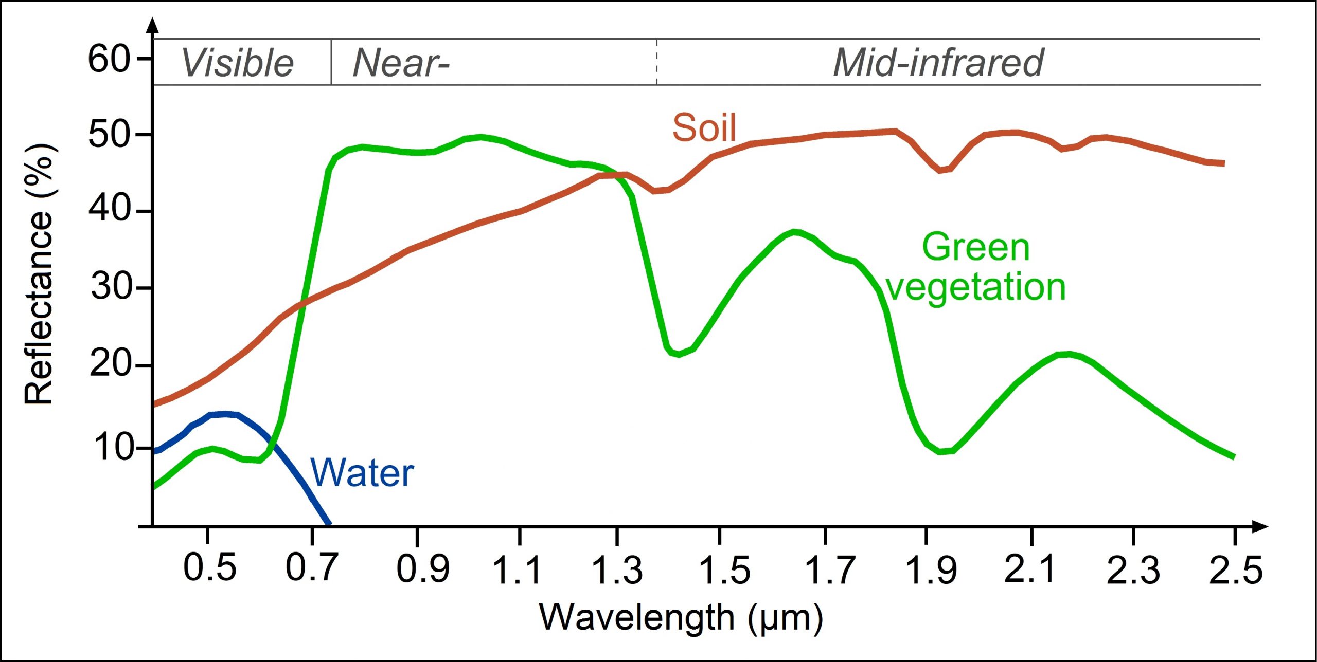
Visible wavelength region
Healthy green vegetation absorbs most of the visible light incident on it, using it to grow through the process of photosynthesis. Photosynthesis is a relatively complex biochemical process that begins with the absorption of a photon by a pigment molecule, which sets off an electronic transition (the movement of an electron from one energy level to a higher one) that starts a chain-reaction leading to production of plant material from the basic chemical components of CO2 and water. A form of chlorophyll is the dominant pigment in almost all vegetation, and chlorophyll is very good at absorbing visible light, which is why vegetation has low reflectances across the visible wavelengths. Chlorophyll is a little better at absorbing blue and red wavelengths than it is at absorbing green wavelengths, so relatively more of the green radiation is reflected, giving vegetation its green appearance.
Infrared wavelength region
Incoming photons at wavelengths in the near-infrared region individually contain less energy (recall that the energy in a photon is proportional to its frequency, and hence inversely proportional to its wavelength). These photons are therefore unable to cause an electronic transition so pigments used for photosynthesis cannot use them, and in general do not absorb them. Other parts of plants, especially liquid water found in the leaves, do absorb these photons, which rotate and stretch chemical bonds in the water or in plant cells, effectively heating up the absorbing material. In general, plants have no need for heating up, and except for wavelengths around 1.4 μm and 1.9 μm where water is a strong absorber, plants reflect much of the incoming near-infrared radiation.
The combination of low reflectance in the visible and high reflectance in the near-infrared wavelengths is the most characteristic signature of vegetation used in remote sensing, and is used for quick-and-dirty mapping of vegetation on Earth. Consider that most land areas contain a mix of vegetated and unvegetated areas. Sometimes this ‘mix’ is very one-sided, as in the Amazon, the Sahara desert, or the Canadian Arctic, and sometimes it is truly more mixed, as on the African savanna (Figure 68).
Vegetation indices
Using the reflectance in the visible wavelengths alone does not tell us how much vegetation is in an area, because water also has low reflectance in this wavelength region. And using the reflectance in the near-infrared region alone also does not tell us much about vegetation, because other surface types, such as the bright sand and bright snow depicted in Figure 68 also have higher near-infrared reflectance. However, the ratio of the visible and near-infrared reflectances is a useful indicator for the amount of vegetation present in an area because no other surface type has both as high near-infrared and as low visible reflectance as vegetation. This observation led initially to the development of what is called the Simple Ratio (SR):
where NIR is the surface reflectance in the near-infrared wavelength region (typically around 700-1000 nm), and RED is the same for the red wavelength region (600-700 nm).
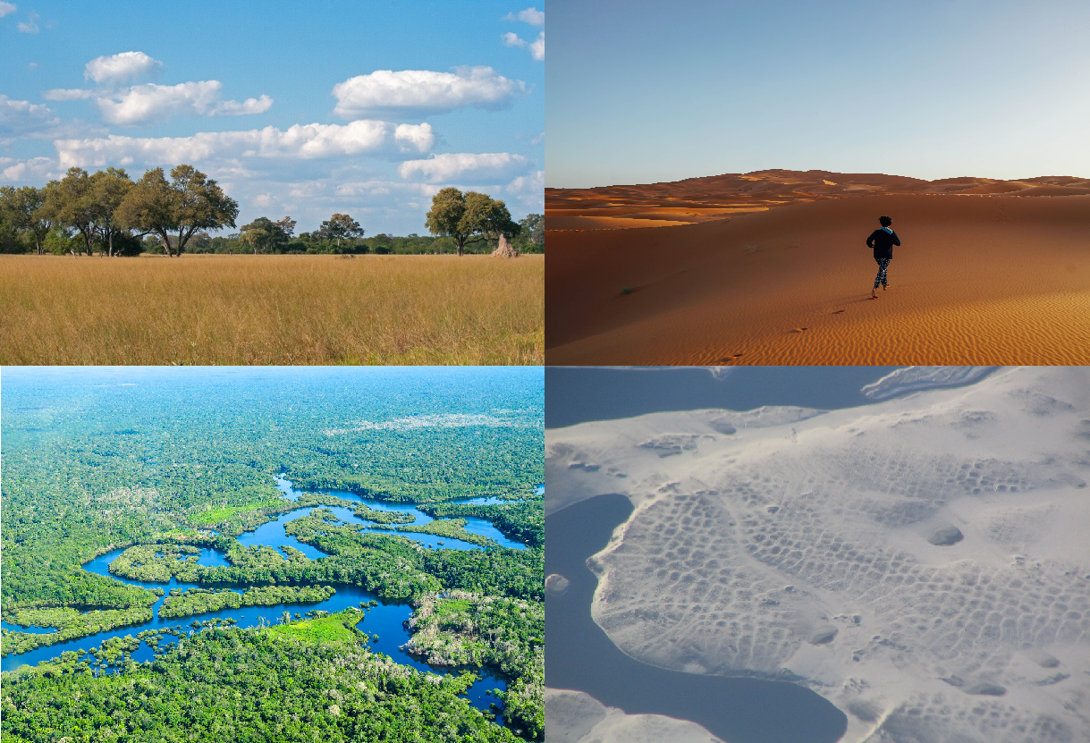
68: Four areas with rather different vegetation characteristics. Top left: The African savanna contain a mix of trees and grass cover. Trees On The African Savanna by Lynn Greyling, PublicDomainPictures.net, CC0 1.0. Top right: The Sahara desert is in most places void of vegetation. Sahara Desert by Azer Koçulu, Wikimedia Commons, CC0 1.0. Bottom left: The Amazon rainforest is covered in dense vegetation. Amazon Rainforest by CIFOR (Neil Palmer/CIAT), Flickr, CC BY-NC-ND 2.0. Bottom right: The Canadian Arctic has large areas with no vegetation. Patterned ground in Canadian tundra by Raymond M. Coveney, Wikimedia Commons, CC BY-SA 3.0.
While surface reflectance values should in principle always be used to calculate this and any other vegetation index, in practice these calculations are often done instead based on TOA reflectance or even TOA radiance (or even DN values!). The Simple Ratio has one drawback that means it is rarely used – its values approach infinity when red reflectance approaches zero, which makes differences between large values difficult to interpret. A simple improvement called the Normalized Difference Vegetation Index (NDVI), based on the same two measurements, is therefore more commonly used:
NDVI values range from a minimum of -1 to a maximum of +1. Typical values for bare soil are around 0, for water around -0.2, and for vegetation in the range 0.1-0.7 depending on vegetation health and density. Because NDVI relies only on two measurements, in the near-infrared and red wavelength regions, it can be calculated with data from the earliest multispectral sensors in orbit, including the Landsat series (since 1972) and the AVHRR series (since 1978). This allows easy visualizations of vegetation cover, on small or large scales, such as the one shown in Figure 69.
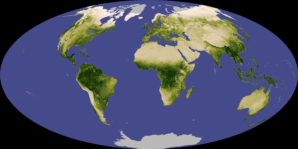
69: NDVI composite of Earth, showing relative differences in vegetation cover. Globalndvi tmo 200711 lrg by Reto Stockli and Jesse Allen (NASA), Wikimedia Commons, public domain.
Vegetation indices can be used for more than producing pretty pictures of global vegetation distribution. As a result of global warming, which is especially pronounced in the Arctic region, the northern parts of Canada are undergoing rapid changes in vegetation distribution and growth patterns. Monitoring such changes over this large and very sparsely populated region is based on long-term NDVI trends in the summer months, which among other things demonstrates that region undergoing faster warming also experience more rapid growth in vegetation density. Another important use of vegetation indices is in crop yield forecasting: by tracking NDVI through an agricultural growing season, the development of the crops can be quantified and their eventual yields predicted statistically. Probably the most important use of such crop prediction models is to forecast droughts, crop failures and famines in parts of the world where people depend on local agriculture for their food supply. This is done systematically for countries that are prone to famine by the Famine Early Warning Systems Network (FEWS), a US-based organization, and it is also done by many national governments and regional/global organizations. Vegetation indices thus literally have the potential to save lives – if the global community responds to the predictions generated by them.
Many refinements have been introduced since the development of NDVI, to create vegetation indices that perform better under a range of conditions. These include the Soil-Adjusted Vegetation Index, the Enhanced Vegetation Index used with MODIS data, and the Global Vegetation Index used with MERIS data. These newer vegetation indices were specifically designed to be more robust to varying environmental conditions, such as variations in soil brightness and atmospheric conditions. Despite such refinements, all vegetation indices suffer from a fundamental drawback: while their interpretation is quite clear in relative terms (higher values indicate more green vegetation), their relationship to real measureable vegetation characteristics used by people outside the field of remote sensing is not clear.
A vegetation index not intended to portray vegetation density, but rather to portray relative differences in vegetation water content, has been developed specifically to take advantage of the water absorption feature around 1.4 μm shown in Figure 67. It is called the Normalized Difference Water Index (NDWI), and its generic equation is:
where SWIR denotes a measurement in the short-wave infrared region (1.4 μm). Dry vegetation contains less water, and therefore absorbs less of the SWIR radiation, reducing the value of NDWI.
For any vegetation index, the specific bands that are used as the ‘RED’, ‘NIR’ and ‘SWIR’ bands depends on the sensor in question, and not all sensors have bands appropriate for calculating one or another index.
Mapping real vegetation attributes
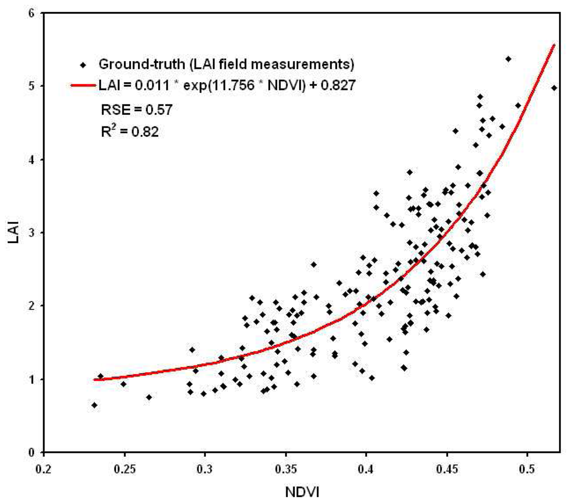
Vegetation attributes that are more used by non-remote sensing people include among other things above-ground biomass, absorbed photosynthetically active radiation (APAR), and the Leaf Area Index (LAI). Above-ground biomass can be measured (by cutting and weighing it) in kg/ha, and is of fundamental interest in monitoring vegetation trends. APAR is the amount of radiation that is absorbed by vegetation (per areal unit), and is strongly linked to vegetation growth and crop yield. LAI is the (one-sided) area of leaves divided by the area of ground, so it is a unitless measure of leaf density. Because (water and) gas exchange between vegetation and the atmosphere happens through the leaves, LAI can be used as a proxy for this exchange, which is important for vegetation’s function as a carbon sink, among other things. All of these vegetation attributes are thus more directly linked to the function of vegetation in the environment, and certainly more directly interpretable, than is a vegetation index. But they are also much more difficult to map with remote sensing data.
Empirical approach
A simple approach to mapping LAI is illustrated in Figure 70, in which NDVI values have been regressed against field-measured LAI. As is obvious from Figure 70, what we measure in remote sensing data is related, but not very closely, and certainly not linearly, to actual LAI measured on the ground. Nevertheless the regression lines can be used to produce a first approximation of LAI from these remote sensing data. A similar approach can be taken to map other vegetation attributes.
Radiative transfer approach
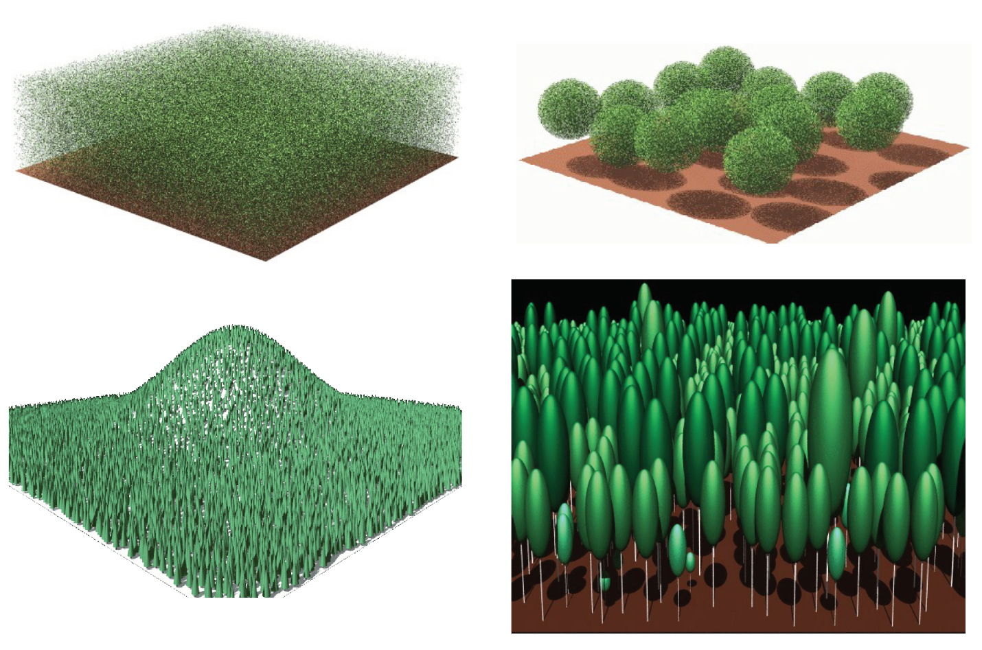
More sophisticated approaches to mapping vegetation attributes rely on radiative transfer models. Radiative transfer models build up a simple 3D world consisting of a) the ground, b) some vegetation on the ground, c) the atmosphere, and d) the Sun. Each of these elements have specific attributes that define how they interact with radiation: The Sun emits a certain amount of radiation at each modeled wavelength, the atmosphere absorbs and scatters this radiation to some degree, and the vegetation and the ground absorb and reflect the radiation. Once specified, the model can then be ‘run’ to determine what the TOA radiance (or other measureable radiation parameter) would be for a given combination on element definition. These elements can then be changed and the model ‘run’ again to see how the change affects the TOA radiance. For example, different densities of vegetation can be included, representing different values of LAI, each producing a unique combination of TOA radiances in different wavelengths. To produce a robust picture of how LAI influences TOA radiance, the other elements must also be varied, so the influence of soil colour and atmospheric constituents also get captured in the process. Even more importantly, non-LAI variation in vegetation must also be considered. Individual leaves may have different spectral signatures depending on their pigment composition, leaves of different shapes and orientation interact with the Sun’s radiation differently, and the structure of the canopy also exerts its own influence (e.g. are the leaves distributed randomly, evenly, or in a clumped manner?). Varying all of these parameters, each time running the radiative transfer model to determine what their specific combination would look like at the top of the atmosphere, allows you to build up a look-up table with a) environmental conditions including the parameter of interest (e.g. LAI) and b) the resulting TOA (spectral) radiance. When mapping LAI with a satellite image, the observed TOA radiance of each pixel can then be matched to the entry in the table it matches most closely to determine the probably value of LAI in that pixel.
Fire
Another sub-field of remote sensing concerns mapping of fire. Active fire is relatively easily detected because it is hot, and heat can be detected with thermal sensors, and because it creates smoke, and smoke is visible in satellite imagery. Detecting active fire with satellite data is so well-developed that a near-instantaneous ‘active fire product’ is made each time a MODIS or VIIRS sensor passes over an area.
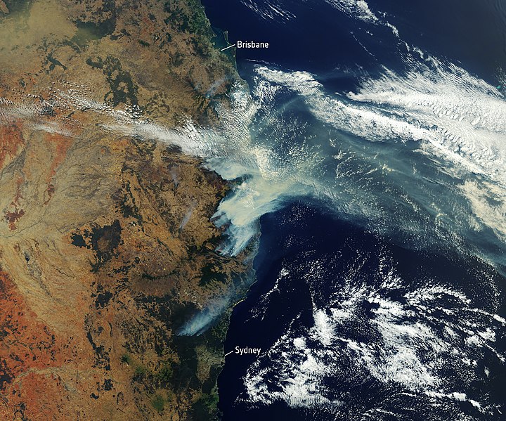
72: Example of active fire detection from space during the Australian wildfires of 2019. Satellite image of bushfire smoke over Eastern Australia by the European Space Agency, Flickr, CC BY-SA 2.0.
Once a fire is over, it may be important to assess how much area was burned, and how intensely it was burned. This has important implications for the recovery of the vegetation and associated biota in the area, and it can also help us answer important questions related to climate change, like how the frequency, duration, size, and intensity of wildfires are changing as the climate warms. While there are different ways to assess these parameters, the most commonly used approach involves quantifying something called the Normalized Burn Ratio (NBR). The NBR is calculated as:
which, you might say, is the same as the definition of NDWI! And it is close, but the term SWIR covers a fairly wide range of wavelengths, and while for NDWI the original definition of ‘SWIR’ referred to wavelengths around 1.24 μm, for NBR ‘SWIR’ was specifically designed for band 7 on Landsat 4 and 5, which is centered around 2.2 μm. Nevertheless, NBR is really just a vegetation index, and while it is not the only index one can use for mapping fire impacts, and not even necessarily the best one, it is the most commonly used. To use it for quantification of fire severity, one needs to compare NBR values in two images, one from before and one from after the fire, which leads to the calculation of δNBR:
To minimize the effects of other environmental factors on this calculation, it is ideal to use ‘anniversary dates’ to calculate δNBR, although this is not necessary if two images are available from a small period covering just before and just after the fire (Figure 73).
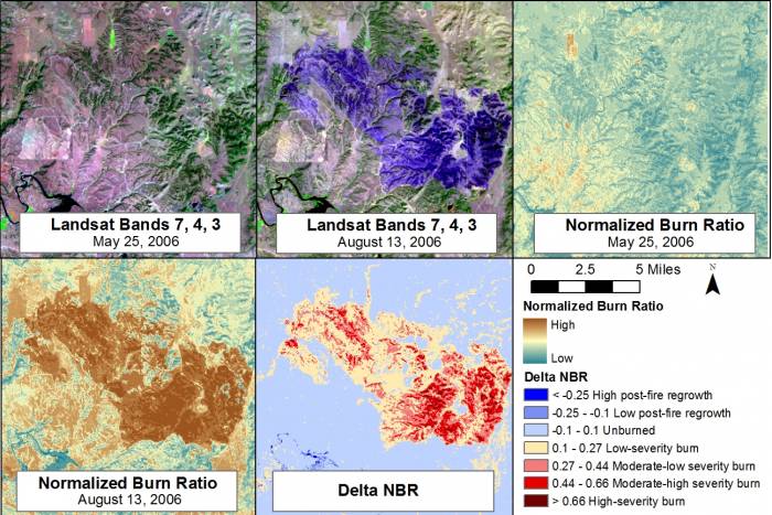
73: Example of a pre-fire image (top left), a post-fire image (top middle), pre-fire NBR (top right), post-fire NBR (bottom left), and δNBR (bottom middle). While the impact of the fire is evident in the original imagery, the use of δNBR helps highlight the difference between the two images. Example of normalized burn ratio from a fire at Camp Gurnsey, Wyoming in 2006 by Jason Karl, The Landscape Toolbox, CC0 1.0.
Because NBR is calculated as a normalized difference, its values range between -1 and +1, so δNBR ranges, in theory, from -2 to +2, with higher values indicating greater fire severity. As with other vegetation indices, extreme values are rare though, so even values of 0.2-0.3 indicate relatively severe fire impacts.
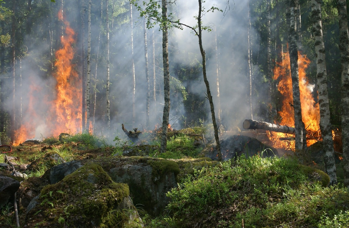
74: An example of both vegetation and fire, both of which can be mapped well with remote sensing. Forest Fire, by YIvers, Pixabay, Pixabay License.