
7: National Spatial Data Infrastructure II
- Page ID
- 8173

National Spatial Data Infrastructure II
David DiBiase
7.1. Overview
Chapters 6 and 7 consider the origins and characteristics of the framework data themes that make up the United States’ proposed National Spatial Data Infrastructure (NSDI). Chapter 6 discussed the geodetic control and orthoimagery themes. This chapter describes the origins, characteristics and current status of the elevation, transportation, hydrography, governmental units and cadastral themes.
Objectives
Students who successfully complete Chapter 7 should be able to:
- Given a regular or irregular array of spot elevations, construct a triangulated irregular network, interpolate contour intervals and draw contour lines;
- Compare vector and raster representations of terrain elevation;
- Acquire and view digital elevation data from the National Elevation Dataset;
- Calculate an interpolated spot elevation based on neighboring elevations;
- Contrast the characteristics of three global elevation data products;
- Describe the characteristics and current status of the NSDI hydrography, transportation, and governmental units themes as implemented in USGS’ National Map; and
- Interpret the size and relative location of a land parcel designated in terms of the U.S. Public Land Survey System.
Comments and Questions
Registered students are welcome to post comments, questions, and replies to questions about the text. Particularly welcome are anecdotes that relate the chapter text to your personal or professional experience. In addition, there are discussion forums available in the ANGEL course management system for comments and questions about topics that you may not wish to share with the whole world.
To post a comment, scroll down to the text box under “Post new comment” and begin typing in the text box, or you can choose to reply to an existing thread. When you are finished typing, click on either the “Preview” or “Save” button (Save will actually submit your comment). Once your comment is posted, you will be able to edit or delete it as needed. In addition, you will be able to reply to other posts at any time.
Note: the first few words of each comment become its “title” in the thread.
7.2. Checklist
The following checklist is for Penn State students who are registered for classes in which this text, and associated quizzes and projects in the ANGEL course management system, have been assigned. You may find it useful to print this page out first so that you can follow along with the directions.
| Step | Activity | Access/Directions |
|---|---|---|
| 1 | Read Chapter 7 | This is the second page of the Chapter. Click on the links at the bottom of the page to continue or to return to the previous page, or to go to the top of the chapter. You can also navigate the text via the links in the GEOG 482 menu on the left. |
| 2 | Submit 3 practice quizzesincluding:
Practice quizzes are not graded and may be submitted more than once. | Go to ANGEL > [your course section] > Lessons tab > Chapter 7 folder > [quiz] |
| 3 | Perform “Try this” activitiesincluding:
“Try this” activities are not graded. | Instructions are provided for each activity. |
| 4 | Submit theChapter 7 Graded Quiz | ANGEL > [your course section] > Lessons tab > Chapter 7 folder > Chapter 7 Graded Quiz. See the Calendar tab in ANGEL for due dates. |
| 5 | Readcomments and questionsposted by fellow students. Add comments and questions of your own, if any. | Comments and questions may be posted on any page of the text, or in a Chapter-specific discussion forum in ANGEL. |
7.3. Theme: Elevation
The NSDI Framework Introduction and Guide (FGDC, 1997, p. 19) points out that “elevation data are used in many different applications.” Civilian applications include flood plain delineation, road planning and construction, drainage, runoff, and soil loss calculations, and cell tower placement, among many others. Elevation data are also used to depict the terrain surface by a variety of means, from contours to relief shading and three-dimensional perspective views.
The NSDI Framework calls for an “elevation matrix” for land surfaces. That is, the terrain is to be represented as a grid of elevation values. The spacing (or resolution) of the elevation grid may vary between areas of high and low relief (i.e., hilly and flat). Specifically, the Framework Introduction states that
Elevation values will be collected at a post-spacing of 2 arc-seconds (approximately 47.4 meters at 40° latitude) or finer. In areas of low relief, a spacing of 1/2 arc-second (approximately 11.8 meters at 40° latitude) or finer will be sought (FGDC, 1997, p. 18).
The elevation theme also includes bathymetry–depths below water surfaces–for coastal zones and inland water bodies. Specifically,
For depths, the framework consists of soundings and a gridded bottom model. Water depth is determined relative to a specific vertical reference surface, usually derived from tidal observations. In the future, this vertical reference may be based on a global model of the geoid or the ellipsoid, which is the reference for expressing height measurements in the Global Positioning System (Ibid).
USGS has lead responsibility for the elevation theme. Elevation is also a key component of USGS’ National Map. The next several pages consider how heights and depths are created, how they are represented in digital geographic data, and how they may be depicted cartographically.
7.4. Vector and Raster Approaches
The terms raster and vector were introduced back in Chapter 1 to denote two fundamentally different strategies for representing geographic phenomena. Both strategies involve simplifying the infinite complexity of the Earth’s surface. As it relates to elevation data, the raster approach involves measuring elevation at a sample of locations. The vector approach, on the other hand, involves measuring the locations of a sample of elevations. I hope that this distinction will be clear to you by the end of this chapter.
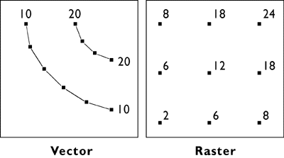
Vector and raster representations of the same terrain surface.
The illustration above compares how elevation data are represented in vector and raster data. On the left are elevation contours, a vector representation that is familiar with anyone who has used a USGS topographic map. The technical term for an elevation contour isisarithm, from the Greek words for “same” and “number.” The termsisoline, isogram, and isopleth all mean more or less the same thing. (See any cartography text for the distinctions.)
As you will see later in this chapter, when you explore Digital Line Graph hypsography data using Global Mapper or dlgv 32 Pro, elevations in vector data are encoded as attributes of line features. The distribution of elevation points across the quadrangle is therefore irregular. Raster elevation data, by contrast, consist of grids of points at which elevation is encoded at regular intervals. Raster elevation data are what’s called for by the NSDI Framework and the USGS National Map. Digital contours can now be rendered easily from raster data. However, much of the raster elevation data used in the National Map was produced from digital vector contours and hydrography (streams and shorelines). For this reason we’ll consider the vector approach to terrain representation first.
7.5. Contours
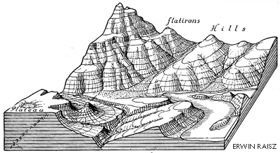
Contour lines trace the elevation of the terrain surface at regularly-spaced intervals (Raisz, 1948. © McGraw-Hill, Inc. Used by permission).
Drawing contour lines is a way to represent a terrain surface with a sample of elevations. Instead of measuring and depicting elevation at every point, you measure only along lines at which a series of imaginary horizontal planes slice through the terrain surface. The more imaginary planes, the more contours, and the more detail is captured.
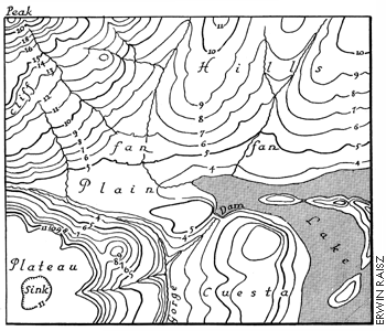
Contour lines representing the same terrain as in the first figure, but in plan view. (Raisz, 1948. © McGraw-Hill, Inc. Used by permission).
Until photogrammetric methods came of age in the 1950s, topographers in the field sketched contours on the USGS 15-minute topographic quadrangle series. Since then, contours shown on most of the 7.5-minute quads were compiled from stereoscopic images of the terrain, as described in Chapter 6. Today computer programs draw contours automatically from the spot elevations that photogrammetrists compile stereoscopically.
Although it is uncommon to draw terrain elevation contours by hand these days, it is still worthwhile to know how. In the next few pages you’ll have a chance to practice the technique, which is analogous to the way computers do it.
7.6. Contouring By Hand
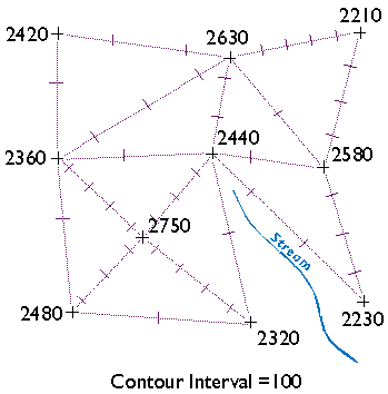
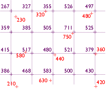
This page will walk you through a methodical approach to rendering contour lines from an array of spot elevations (Rabenhorst and McDermott, 1989). To get the most from this demonstration, I suggest that you print the illustration in the attached image file. Find a pencil (preferably one with an eraser!) and straightedge, and duplicate the steps illustrated below. A “Try This!” activity will follow this step-by-step introduction, providing you a chance to go solo.
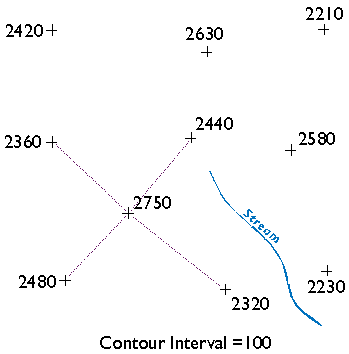
Beginning a triangulated irregular network.
Starting at the highest elevation, draw straight lines to the nearest neighboring spot elevations. Once you have connected to all of the points that neighbor the highest point, begin again at the second highest elevation. (You will have to make some subjective decisions as to which points are “neighbors” and which are not.) Taking care not to draw triangles across the stream, continue until the surface is completely triangulated.

Complete TIN. Note that the triangle sides must not cross hydrologic features (i.e., the stream) on a terrain surface.
The result is a triangulated irregular network (TIN). A TIN is a vector representation of a continuous surface that consists entirely of triangular facets. The vertices of the triangles are spot elevations that may have been measured in the field by leveling, or in a photogrammetrist’s workshop with a stereoplotter, or by other means. (Spot elevations produced photogrammetrically are called mass points.) A useful characteristic of TINs is that each triangular facet has a single slope degree and direction. With a little imagination and practice, you can visualize the underlying surface from the TIN even without drawing contours.
Wonder why I suggest that you not let triangle sides that make up the TIN cross the stream? Well, if you did, the stream would appear to run along the side of a hill, instead of down a valley as it should. In practice, spot elevations would always be measured at several points along the stream, and along ridges as well. Photogrammetrists refer to spot elevations collected along linear features as breaklines (Maune, 2007). I omitted breaklines from this example just to make a point.
You may notice that there is more than one correct way to draw the TIN. As you will see, deciding which spot elevations are “near neighbors” and which are not is subjective in some cases. Related to this element of subjectivity is the fact that the fidelity of a contour map depends in large part on the distribution of spot elevations on which it is based. In general, the density of spot elevations should be greater where terrain elevations vary greatly, and sparser where the terrain varies subtly. Similarly, the smaller the contour interval you intend to use, the more spot elevations you need.
(There are algorithms for triangulating irregular arrays that produce unique solutions. One approach is called Delaunay Triangulationwhich, in one of its constrained forms, is useful for representing terrain surfaces. The distinguishing geometric characteristic of a Delaunay triangulation is that a circle surrounding each triangle side does not contain any other vertex.)
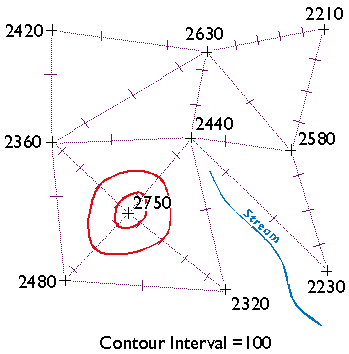
Tick marks drawn where elevation contours cross the edges of each TIN facet.
Now draw ticks to mark the points at which elevation contours intersect each triangle side. For instance, see the triangle side that connects the spot elevations 2360 and 2480 in the lower left corner of the illustration above? One tick mark is drawn on the triangle where a contour representing elevation 2400 intersects. Now find the two spot elevations, 2480 and 2750, in the same lower left corner. Note that three tick marks are placed where contours representing elevations 2500, 2600, and 2700 intersect.
This step should remind you of the equal interval classification scheme you read about in Chapter 3. The right choice of contour interval depends on the goal of the mapping project. In general, contour intervals increase in proportion to the variability of the terrain surface. It should be noted that the assumption that elevations increase or decrease at a constant rate is not always correct, of course. We will consider that issue in more detail later.
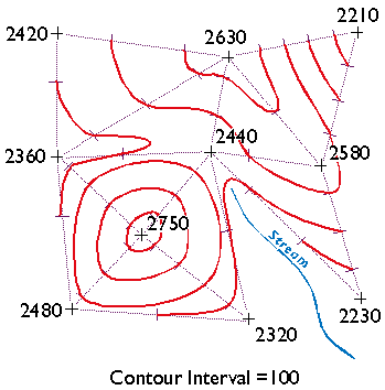
Threading elevation contours through a TIN.
Finally, draw your contour lines. Working downslope from the highest elevation, thread contours through ticks of equal value. Move to the next highest elevation when the surface seems ambiguous.
Keep in mind the following characteristics of contour lines (Rabenhorst and McDermott, 1989):
- Contours should always point upstream in valleys
- Contours should always point downridge along ridges
- Adjacent contours should always be sequential or equivalent
- Contours should never split into two
- Contours should never cross or loop
- Contours should never spiral
- Contours should never stop in the middle of a map
How does your finished map compare with the one I drew below?
TRY THIS !
Now try your hand at contouring on your own. The purpose of this practice activity is to give you more experience in contouring terrain surfaces.
- First, view an image of an irregular array of 16 spot elevations.
- Print the image.
- Use the procedure outlined in this lesson to draw contour lines that represent the terrain surface that the spot elevations were sampled from. You may find this to be a moderately challenging task that takes about a half hour to do well. TIP: label the tick marks to make it easier to connect them.
- When finished, compare your result to an existing map.
Here are a couple of somewhat simpler problems and solutions in case you need a little more practice.
- Practice Problem #1
- Practice Problem #1 Solution
- Practice Problem #2
- Practice Problem #2 Solution
You will be asked to demonstrate your contouring ability again in the Lesson 7 Quiz and in the final exam.
Kevin Sabo (personal communication, Winter 2002) remarked that “If you were unfortunate enough to be hand-contouring data in the 1960′s and 70′s, you may at least have had the aid of a Gerber Variable Scale. After hand contouring in Lesson 7, I sure wished I had my Gerber!”
PRACTICE QUIZ
Registered Penn State students should return now to the Chapter 7 folder in ANGEL (via the Resources menu to the left) to take a self-assessment quiz about Contouring. You may take practice quizzes as many times as you wish. They are not scored and do not affect your grade in any way.
7.7. Digital Line Graph (DLG)
IDENTIFICATION
Digital Line Graphs (DLGs) are vector representations of most of the features and attributes shown on USGS topographic maps. Individual feature sets (outlined in the table below) are encoded in separate digital files. DLGs exist at three scales: small (1:2,000,000), intermediate (1:100,000) and large (1:24,000). Large-scale DLGs are produced intiles that correspond to the 7.5-minute topographic quadrangles from which they were derived.
| Layer | Features |
|---|---|
| Public Land Survey System (PLSS) | Township, range, and section lines |
| Boundaries | State, county, city, and other national and State lands such as forests and parks |
| Transportation | Roads and trails, railroads, pipelines and transmission lines |
| Hydrography | Flowing water, standing water, and wetlands |
| Hypsography | Contours and supplementary spot elevations |
| Non-vegetative features | Glacial moraine, lava, sand, and gravel |
| Survey control and markers | Horizontal and vertical monuments (third order or better) |
| Man-made features | Cultural features, such as building, not collected in other data categories |
| Woods, scrub, orchards, and vineyards | Vegetative surface cover |
Layers and contents of large-scale Digital Line Graph files. Not all layers available for all quadrangles (USGS, 2006).
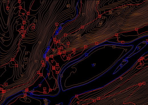
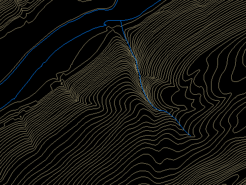
Portion of three Digital Line Graph (DLG) layers for USGS Bushkill, PA quadrangle; imaged with Global Mapper (dlgv32 Pro) software. Transportation features are arbitrarily colored red, hydrography blue, and hypsography brown. The square symbols are nodes and the triangles represent polygon centroids.
DATA QUALITY
Like other USGS data products, DLGs conform to National Map Accuracy Standards. In addition, however, DLGs are tested for the logical consistency of the topological relationships among data elements. Similar to the Census Bureau’s TIGER/Line, line segments in DLGs must begin and end at point features (nodes), and line segments must be bounded on both sides by area features (polygons).
SPATIAL REFERENCE INFORMATION
DLGs are heterogenous. Some use UTM coordinates, others State Plane Coordinates. Some are based on NAD 27, others on NAD 83. Elevations are referenced either to NGVD 29 or NAVD 88 (USGS, 2006a).
ENTITIES AND ATTRIBUTES
The basic elements of DLG files are nodes (positions), line segments that connect two nodes, and areas formed by three or more line segments. Each node, line segment, and area is associated with two-part integer attribute codes. For example, a line segment associated with the attribute code “050 0412″ represents a hydrographic feature (050), specifically, a stream (0412).
DISTRIBUTION
Not all DLG layers are available for all areas at all three scales. Coverage is complete at 1:2,000,000. At the intermediate scale, 1:100,000 (30 minutes by 60 minutes), all hydrography and transportation files are available for the entire U.S., and complete national coverage is planned. At 1:24,000 (7.5 minutes by 7.5 minutes), coverage remains spotty. The files are in the public domain, and can be used for any purpose without restriction.
Large- and Intermediate -scale DLGs are available for download through EarthExplorer system. You can plot 1:2,000,000 DLGs on-line at the USGS’ National Atlas of the United States.
DIGITAL LINE GRAPH HYPSOGRAPHY
In one sense, DLGs are as much “legacy” data as the out-of-date topographic maps from which they were produced. Still, DLG data serve as primary or secondary sources for several themes in the USGS National Map, including hydrography, boundaries, and transportation. DLG hypsography data are not included in the National Map, however. It is assumed that GIS users can generate elevation contours as needed from DEMs. DLG hypsography and hydrography layers are the preferred sources from which USGS DEMs are produced, however.
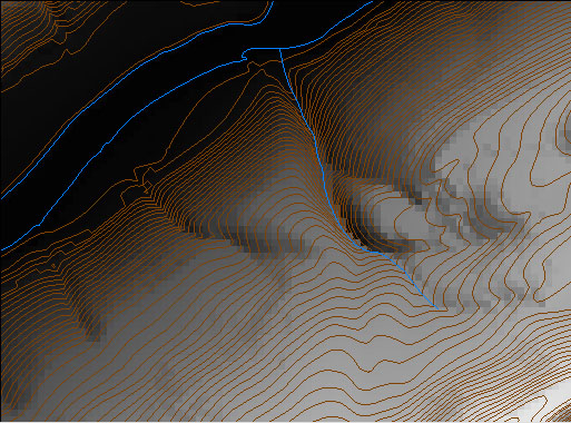
Portion of the hypsography and hydrography layers of a large-scale Digital Line Graph (DLG). USGS Bushkill, PA quadrangle; imaged with Global Mapper (dlgv32 Pro) software.
Hypsography refers to the measurement and depiction of the terrain surface, specifically with contour lines. Several different methods have been used to produce DLG hypsography layers, including:
- Scanning contour lines on photographic film or paper maps, converting the scanned raster data to vectors, then editing and attributing the vector features;
- Manually digitizing and attributing contour lines on photographic film or paper maps; and
- Producing contours by photogrammetric processes.
The preferred method is to manually digitize contour lines in vector mode, then to key-enter the corresponding elevation attribute data.
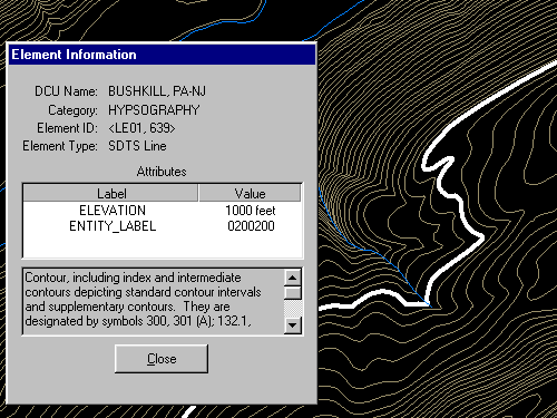
The highlighted contour line has been selected, and its attributes reported in a Global Mapper window. Notice that the line feature is attributed with a unique Element ID code (LE01, 639) and an elevation (1000 feet).
TRY THIS!
EXPLORING DLGS WITH GLOBAL MAPPER (DLGV32 PRO)
Now I’d like you to use Global Mapper (or dlgv32 Pro) software to investigate the characteristics of the hypsography layer of a USGS Digital Line Graph (DLG). The instructions below assume that you have already installed software on your computer. (If you haven’t, return to installation instructions presented earlier in Chapter 6). First you’ll download and a sample DLG file. In a following activity you’ll have a chance to find and download DLG data for your area.
- If you haven’t done so already, create a directory called “USGS Data” on your hard disk, where you file your course materials.
- Next, Download the DLG.zip data archive. The ZIP archive is 1.2 Mb in size and will take approximately 15 seconds to download via high speed DSL or cable, or about 4 minutes and 15 seconds minutes via 56 Kbps modem.
- Now decompress the archive into a directory on your hard disk.
- Open the archive DLG.zip.
- Create a subdirectory called “DLG” within the directory in which you save data for this class.
- Extract all files in the ZIP archive into your new subdirectory.
The end result will be five subdirectories, each of which includes the data files that make up a DLG “layer,” along with a master directory.
- Launch Global Mapper or dlgv32 Pro.
- Open a Digital Line Graph by choosing File > Open as New…, then navigate to the directory “DLG/Hypso.” Open the file ‘Hp01catd.ddf’ (you can open up to four files at once in the trial version of Global Mapper.) The data correspond with the 7.5 minute quadrangle for Bushkill, PA. The file is encoded in Spatial Data Transfer Standard (SDTS) format. For information about SDTS, see the SDTS Tutorial(PDF format).
- Global Mapper may ask you to direct it to a ‘Master Data Dictionary’ file. If so, navigate to, and select, the file ‘Dlg/MasterDlg/Dlg3mdir.ddf’
- Experiment with Global Mapper’s tools. Use Zoom and Pan to magnify and scroll across the DLG. The Full View button (the one with the house icon) refreshes the initial full view of the data set.
- The Feature Info tool allows you to query the attributes of a particular feature. Try clicking a single line segment. Note that you can display the attributes of a feature in the lower left portion of the application window by simply hovering over the feature.
- The Measure tool (ruler icon) allows you to not only measure distance as the crow flies, but also to see the area enclosed by a series of line segments drawn by repeated mouse clicks. Note again the location information that is given to you near the bottom of the application window.
- Certain tools, e.g., the 3D Path Profile/Line of Sight tool (next to the Feature Info tool) are not functional in the free (unregistered) version of Global Mapper.
- The trial version of Global Mapper allows you to open and view up to four files at once. You might find it interesting to open and compare the Bushkill DLG hypsography file and the corresponding DRG you viewed in Lesson 6. Note that you can turn layers on and off, and even adjust their transparency at Tools > Control Center. How do the contours in the DLG compare with those in the DRG? What explains the difference?
- Global Mapper provides the metadata you’ll need to answer questions in a practice quiz. To access the metadata, navigate to Tools > Control Center, then click the Metadata button.
7.8. Digital Elevation Model (DEM)
The term “Digital Elevation Model” has both generic and specific meanings. In general, a DEM is any raster representation of a terrain surface. Specifically, a DEM is a data product of the U.S. Geological Survey. Here we consider the characteristics of DEMs produced by the USGS Later in this chapter we’ll consider sources of global terrain data.
IDENTIFICATION
USGS DEMs are raster grids of elevation values that are arrayed in series of south-north profiles. Like other USGS data, DEMs were produced originally in tiles that correspond to topographic quadrangles. Large scale (7.5-minute and 15-minute), intermediate scale (30 minute), and small scale (1 degree) series were produced for the entire U.S. The resolution of a DEM is a function of the east-west spacing of the profiles and the south-north spacing of elevation points within each profile.
DEMs corresponding to 7.5-minute quadrangles are available at 10-meter resolution for much, but not all, of the U.S. Coverage is complete at 30-meter resolution. In these large scale DEMs elevation profiles are aligned parallel to the central meridian of the local UTM zone, as shown in the illustration below. See how the DEM tile in the illustration below appears to be tilted? This is because the corner points are defined in unprojected geographic coordinates that correspond to the corner points of a USGS quadrangle. The farther the quadrangle is from the central meridian of the UTM zone, the more it is tilted.
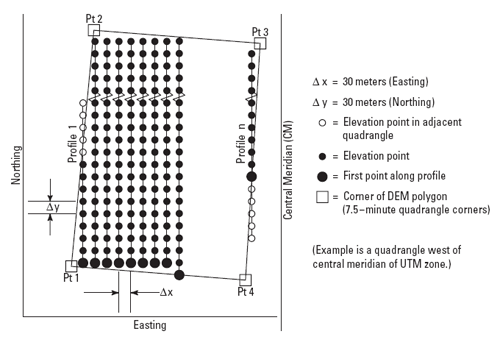
Arrangement of elevation profiles in a large scale USGS Digital Elevation Model (USGS, 1987).
As shown below, the arrangement of the elevation profiles is different in intermediate- and small-scale DEMs. Like meridians in the northern hemisphere, the profiles in 30-minute and 1-degree DEMs converge toward the north pole. For this reason the resolution of intermediate- and small-scale DEMs (that is to say, the spacing of the elevation values) is expressed differently than for large-scale DEMs. The resolution of 30-minute DEMs is said to be 2 arc seconds and 1-degree DEMs are 3 arc seconds. Since an arc second is 1/3600 of a degree, elevation values in a 3 arc second DEM are spaced 1/1200 degree apart, representing a grid cell about 66 meters “wide” by 93 meters “tall” at 45º latitude.
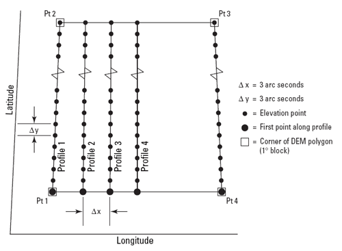
Arrangement of elevation profiles in a small scale USGS Digital Elevation Model (USGS, 1987).
The preferred method for producing the elevation values that populate DEM profiles is interpolation from DLG hypsography and hydrography layers (including the hydrography layer enables analysts to delineate valleys with less uncertainty than hypsography alone). Some older DEMs were produced from elevation contours digitized from paper maps or during photogrammetric processing, then smoothed to filter out errors. Others were produced photogrammtrically from aerial photographs.
DATA QUALITY
The vertical accuracy of DEMs is expressed as the root mean square error (RMSE) of a sample of at least 28 elevation points. The target accuracy for large-scale DEMs is seven meters; 15 meters is the maximum error allowed.
SPATIAL REFERENCE INFORMATION
Like DLGs, USGS DEMs are heterogenous. They are cast on the Universal Transverse Mercator projection used in the local UTM zone. Some DEMs are based upon the North American Datum of 1983, others on NAD 27. Elevations in some DEMs are referenced to either NGVD 29 or NAVD 88.
ENTITIES AND ATTRIBUTES
Each record in a DEM is a profile of elevation points. Records include the UTM coordinates of the starting point, the number of elevation points that follow in the profile, and the elevation values that make up the profile. Other than the starting point, the positions of the other elevation points need not be encoded, since their spacing is defined. (Later in this lesson you’ll download a sample USGS DEM file. Try opening it in a text editor to see what I’m talking about.)
DISTRIBUTION
DEM tiles are available for free download through many state and regional clearinghouses. You can find these sources by searching theGEODATA portion of the Data.Gov site, formerly the separate Geospatial One Stop site.
As part of its National Map initiative, the USGS has developed a “seamless” National Elevation Dataset that is derived from DEMs, among other sources. NED data are available at three resolutions: 1 arc second (approximately 30 meters), 1/3 arc second (approximately 10 meters), and 1/9 arc second (approximately 3 meters). Coverage ranges from complete at 1 arc second to extremely sparse at 1/9 arc second. An extensive FAQ on NED data is published here. The second of the two following activities involves downloading NED data and viewing it in Global Mapper.
TRY THIS!
EXPLORING DEMS WITH GLOBAL MAPPER (DLGV32 PRO)
Global Mapper time again! This time you’ll investigate the characteristics of a USGS DEM. The instructions below assume that you have already installed the software on your computer. (If you haven’t, return to installation instructions presented earlier in Chapter 6). The instructions will remind you how to open a DEM in dlgv32 Pro. In the practice quiz that follows you’ll be asked questions require you to explore the data for answers.
- First Download the DEM.zip data archive. The ZIP archive is 2.5 Mb in size and will take about 30 seconds to download via high speed DSL or cable, or nearly 9 minutes via 56 Kbps modem. If you can’t download the file, contact my teaching assistant or me right away so we can help you resolve the problem.
- Now decompress the archive into a directory on your hard disk.
- Open the archive DEM.zip.
- Create a subdirectory called “DEM” within the directory in which you save class data.
- Extract all files in the ZIP archive into your new subdirectory.
The end result will be two subdirectories, one of which contains a 30-meter DEM, the other a 10-meter DEM. These datasets are in the earlier distribution format of USGS DEM data — elevation data in horizontal (pixel) units of meters and representative of the area covered by a 1:24,000 topo map sheet. In the Try This that follows this one you will see that the distribution format options have expanded.
- Launch Global Mapper.
- Open a Digital Elevation Model by choosing File > Open Data File(s)…, then navigate to the directory DEM_30m or DEM_10m, then open the file bushkill_pa.dem
- Use the Zoom and Pan tools to magnify and scroll across the DEM. The Full View button (house icon) refreshes the initial full view of the dataset.
- Global Mapper provides access to the metadata you’ll need to answer questions in a practice quiz. To access the metadata, navigate to Tools > Control Center, then click the Metadata button.
You can change the appearance of the DEM in the Options section of the Control Center. You can also alter the appearance of the DEM by choosing Tools > Configure, and changing the settings in, especially, Vertical Options and Shader Options. To see the DEM data with(out) hill shading, find the Enable/Disable Hill Shading button on the Shader toolbar (it has a sunburst in the lower left corner).
TRY THIS!
DOWNLOAD YOUR OWN NATIONAL ELEVATION DATASET (NED) DATA
- Go to the Elevation page of the USGS National Map site.
Read any of the information there that you choose. - Follow the link to The National Map Viewer.
If you wish, also follow the link to the detailed instructions that you see under The National Map Viewer link. The following instructions in this Try This should also suffice, and perhaps elaborate at bit more.You will not see Elevation data listed in the left hand Overlays pane. The USGS is in the process of adding more visualization options when it comes to elevation data. See the Hill Shade button at the upper right of the map area. - Use the GIS tools, found above the map area, to pan to and zoom in on an area of interest. Then, click the Download Data button.
Choose a reference area from the pick list. The default is the index of the areas covered by the 1:24,000 topo map series.
You could also chose the entire current map extent, but depending upon your zoom level that may be a huge dataset.
The instructions found via the Help link mentioned above mention that you can define an area based on creating a custom polygon, but at this point I do not see how that is done… - Then click on the map to highlight a specific area of interest. A link to the available data sets will appear in the left hand pane under theSelection tab. (The All Results button will list the multiple areas you click on.) Follow the Download link of the area you are interested in.
- In the USGS Available Data window that opens, select Elevationfrom the Theme column, and choose a file format from the pick list in the Format column.
I know that both the GeoTIFF and ArcGRID formats are compatible with Global Mapper. (ArcGRID is the Esri company’s raster format. You’ll be using the Esri software in future courses.)
Click the Next button. - You will be given a list of Elevation Product choices.
The choices that show Dynamic as the Type will be those that match the Format choice you made in the previous window. The other Stageddatasets are prepackaged and in the formats stated in the Product column, and apparently listed regardless of the Format choice you made.If multiple resolutions are available they will be listed.From the Product list, check the box for what you wish to download.
Click the Next button.
Go to the Cart pane on the right. (It may open automatically.)
Go to Checkout, supply your e-mail address, and submit your order via the Place Order button.
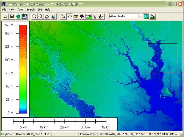
You will receive a message telling you that your order has been placed, and that will soon be followed by an e-mail regarding your order. About an hour and a half after I submitted my request I received a second e-mail containing a download link. - The system will produce a ZIP archive that you can save to your hard disk (e.g., “09647011.zip”)
- Launch Global Mapper and open the ZIP archive. The software can read the data even in its compressed form; you should not need to extract the contents from the .zip file. (It would be a good idea to look at the contents of the .zip archive, though, if only to see the number and type of files included.)
- An image of the DEM data should appear in the Global Mapper window, similar to what you see shown below (even though the image below is from an older version of Global Mapper).
- Again, you can view the metadata associated with the DEM data via the Tools > Control Center menu. Note the PIXEL dimensions reported in arc degrees, as opposed to something like meters.
PRACTICE QUIZ
Registered Penn State students should return now to the Chapter 7 folder in ANGEL (via the Resources menu to the left) to take a self-assessment quiz about DLGs and DEMs. You may take practice quizzes as many times as you wish. They are not scored and do not affect your grade in any way.
7.9. Interpolation
DEMs are produced by various methods. The method preferred by USGS is to interpolate elevations grids from the hypsography and hydrography layers of Digital Line Graphs.
A USGS 7.5-minute DEM and the DLG hypsography and hydrography layers from which it was produced.
The elevation points in DLG hypsography files are not regularly spaced. DEMs need to be regularly spaced to support the slope, gradient, and volume calculations they are often used for. Grid point elevations must be interpolated from neighboring elevation points. In the figure below, for example, the gridded elevations shown in purple were interpolated from the irregularly spaced spot elevations shown in red.
Elevation values in DEMs are interpolated from irregular arrays of elevations measured through photogrammetric methods, or derived from existing DLG hypsography and hydrography data.
Here’s another example of interpolation for mapping. The map below shows how 1995 average surface air temperature differed from the average temperature over a 30-year baseline period (1951-1980). The temperature anomalies are depicted for grid cells that cover 3° longitude by 2.5° latitude.
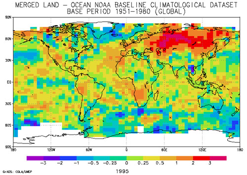
1995 Surface Temperature Anomalies. (National Climatic Data Center, 2005).
The gridded data shown above were estimated from the temperature records associated with the very irregular array of 3,467 locations pinpointed in the map below. The irregular array is transformed into a regular array through interpolation. In general, interpolation is the process of estimating an unknown value from neighboring known values.
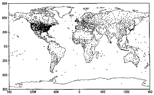
The Global Historical Climate Network. (Eischeid et al., 1995).
Elevation data are often not measured at evenly-spaced locations. Photogrammetrists typically take more measurements where the terrain varies the most. They refer to the dense clusters of measurements they take as “mass points.” Topographic maps (and their derivatives, DLGs) are another rich source of elevation data. Elevations can be measured from contour lines, but obviously contours do not form evenly-spaced grids. Both methods give rise to the need for interpolation.
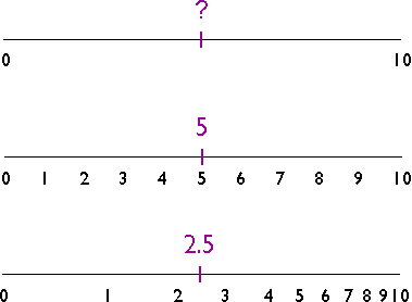
Interpolating an intermediate value on a number line.
The illustration above shows three number lines, each of which ranges in value from 0 to 10. If you were asked to interpolate the value of the tick mark labeled “?” on the top number line, what would you guess? An estimate of “5″ is reasonable, provided that the values between 0 and 10 increase at a constant rate. If the values increase at a geometric rate, the actual value of “?” could be quite different, as illustrated in the bottom number line. The validity of an interpolated value depends, therefore, on the validity of our assumptions about the nature of the underlying surface.
As I mentioned in Chapter 1, the surface of the Earth is characterized by a property called spatial dependence. Nearby locations are more likely to have similar elevations than are distant locations. Spatial dependence allows us to assume that it’s valid to estimate elevation values by interpolation.
Many interpolation algorithms have been developed. One of the simplest and most widely used (although often not the best) is theinverse distance weighted algorithm. Thanks to the property of spatial dependence, we can assume that estimated elevations are more similar to nearby elevations than to distant elevations. The inverse distance weighted algorithm estimates the value z of a point P as a function of the z-values of the nearest n points. The more distant a point, the less it influences the estimate.
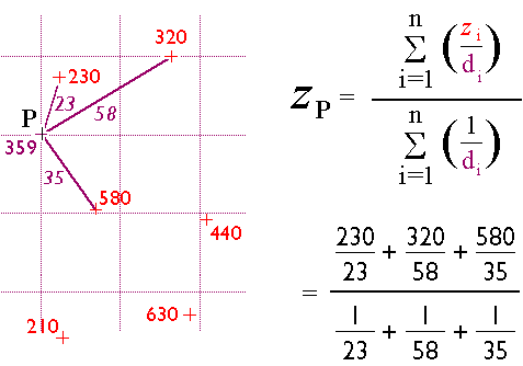
The inverse distance weighted interpolation procedure.
PRACTICE QUIZ
Registered Penn State students should return now to the Chapter 7 folder in ANGEL (via the Resources menu to the left) to take a self-assessment quiz about Interpolation. You may take practice quizzes as many times as you wish. They are not scored and do not affect your grade in any way.
7.10. Slope
Slope is a measure of change in elevation. It is a crucial parameter in several well-known predictive models used for environmental management, including the Universal Soil Loss Equation and agricultural non-point source pollution models.
One way to express slope is as a percentage. To calculate percent slope, divide the difference between the elevations of two points by the distance between them, then multiply the quotient by 100. The difference in elevation between points is called the rise. The distance between the points is called the run. Thus, percent slope equals (rise / run) x 100.
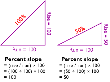
Calculating percent slope. A rise of 100 feet over a run of 100 feet yields a 100 percent slope. A 50-foot rise over a 100-foot run yields a 50 percent slope.
Another way to express slope is as a slope angle, or degree of slope. As shown below, if you visualize rise and run as sides of a right triangle, then the degree of slope is the angle opposite the rise. Since degree of slope is equal to the tangent of the fraction rise/run, it can be calculated as the arctangent of rise/run.
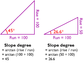
A rise of 100 feet over a run of 100 feet yields a 45° slope angle. A rise of 50 feet over a run of 100 feet yields a 26.6° slope angle.
You can calculate slope on a contour map by analyzing the spacing of the contours. If you have many slope values to calculate, however, you will want to automate the process. It turns out that slope calculations are much easier to calculate for gridded elevation data than for vector data, since elevations are more or less equally spaced in raster grids.
Several algorithms have been developed to calculate percent slope and degree of slope. The simplest and most common is called theneighborhood method. The neighborhood method calculates the slope at one grid point by comparing the elevations of the eight grid points that surround it.
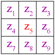
The neighborhood algorithm estimates percent slope in cell 5 by comparing the elevations of neighboring grid cells.
The neighborhood algorithm estimates percent slope at grid cell 5 (Z5) as the sum of the absolute values of east-west slope and north-south slope, and multiplying the sum by 100. The diagram below illustrates how east-west slope and north-south slope are calculated. Essentially, east-west slope is estimated as the difference between the sums of the elevations in the first and third columns of the 3 x 3 matrix. Similarly, north-south slope is the difference between the sums of elevations in the first and third rows (note that in each case the middle value is weighted by a factor of two).
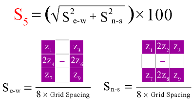
The neighborhood algorithm for calculating percent slope.
The neighborhood algorithm calculates slope for every cell in an elevation grid by analyzing each 3 x 3 neighborhood. Percent slope can be converted to slope degree later. The result is a grid of slope values suitable for use in various soil loss and hydrologic models.
7.11. Relief Shading
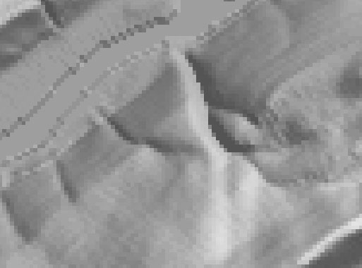
You can see individual pixels in the zoomed image of a 7.5-minute DEM below. I used dlgv32 Pro’s “Gradient Shader” to produce the image. Each pixel represents one elevation point. The pixels are shaded through 256 levels of gray. Dark pixels represent low elevations, light pixels represent high ones.

A digital elevation model in which light pixels represent high elevations, and dark pixels represent low elevations.
It’s also possible to assign gray values to pixels in ways that make it appear that the DEM is illuminated from above. The image below, which shows the same portion of the Bushkill DEM as the image above, illustrates the effect, which is called terrain shading, hill shading or shaded relief.
Shaded terrain image produced from the same DEM as shown in the above figures, using dlgv32 Pro’s Daylight Shader option, with the Surface Color set to gray.
The appearance of a shaded terrain image depends on several parameters, including vertical exaggeration. Click the buttons under the image below to compare the four terrain images of North America shown below, in which elevations are exaggerated 5 times, 10 times, 20 times, and 40 times respectively. (You will need to have the Adobe Flash player installed in order to complete this exercise. If you do not already have the Flash player, you can download it for free from Adobe.)
Effects of vertical exaggeration on a shaded terrain image
Another influential parameter is the angle of illumination. Click the buttons to compare terrain images that have been illuminated from the northeast, southeast, southwest, and northwest. Does the terrain appear to be inverted in one or more of the images? To minimize the possibility of terrain inversion, it is conventional to illuminate terrain from the northwest.
Effects of illumination angle on a shaded terrain image.
7.12. Lidar
For many applications, 30-meter DEMs whose vertical accuracy is measured in meters are simply not detailed enough. Greater accuracy and higher horizontal resolution can be produced by photogrammetric methods, but precise photogrammetry is often too time-consuming and expensive for extensive areas. Lidar is a digital remote sensing technique that provides an attractive alternative.
Lidar stands for LIght Detection And Ranging. Like radar (RAdio Detecting And Ranging), lidar instruments transmit and receive energy pulses, and enable distance measurement by keeping track of the time elapsed between transmission and reception. Instead of radio waves, however, lidar instruments emit laser light (laser stands for Light Amplifications by Stimulated Emission of Radiation).
Lidar instruments are typically mounted in low altitude aircraft. They emit up to 5,000 laser pulses per second, across a ground swath some 600 meters wide (about 2,000 feet). The ground surface, vegetation canopy, or other obstacles reflect the pulses, and the instrument’s receiver detects some of the backscatter. Lidar mapping missions rely upon GPS to record the position of the aircraft, and upon inertial navigation instruments (gyroscopes that detect an aircraft’s pitch, yaw, and roll) to keep track of the system’s orientation relative to the ground surface.
In ideal conditions, lidar can produce DEMs with 15-centimeter vertical accuracy, and horizontal resolution of a few meters. Its cost is prohibitive for small missions, but is justified for larger projects in which detail is essential. For example, lidar has been used successfully to detect subtle changes in the thickness of the Greenland ice sheet that result in a net loss of over 50 cubic kilometers of ice annually.
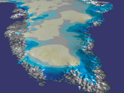
Image of Greenland, viewed from the south, showing changes in ice thickness measured by airborne lidar. Ice sheet thickness decreasing at 40-60 cm per year in darker blue areas (Goddard Space Flight Center, n.d.).
To learn more about the use of lidar in mapping changes in the Greenland ice sheet, visit NASA’s Scientific Visualization Studio.
7.13. Global Elevation Data
This page profiles three data products that include elevation (and, in one case, bathymetry) data for all or most of the Earth’s surface.
ETOPO1
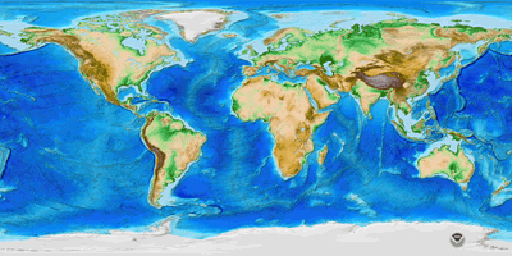
Shaded and colored terrain image produced from ETOPO1 data. (National Geophysical Data Center, 2009).
ETOPO1 is a digital elevation model that includes both topography and bathymetry for the entire world. It consists of more than 233 million elevation values which are regularly spaced at 1 minute of latitude and longitude. At the equator, the horizontal resolution of ETOPO1 is approximately 1.85 kilometers. Vertical positions are specified in meters, and there are two versions of the dataset: one with elevations at the “Ice Surface” of the Greenland and Antarctic ice sheets, and one with elevations at “Bedrock” beneath those ice sheets. Horizontal positions are specified in geographic coordinates (decimal degrees). Source data, and thus data quality, vary from region to region.
You can download ETOPO1 data from the National Geophysical Data Center.
GTOPO30
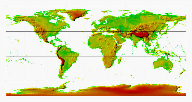
Shaded and colored terrain image produced from GTOPO30 data. Data are distributed as 33 tiles (USGS, 2006b).
GTOPO30 is a digital elevation model that extends over the world’s land surfaces (but not under the oceans). GTOPO30 consists of more than 2.5 million elevation values, which are regularly spaced at 30 seconds of latitude and longitude. At the equator, the resolution of GTOPO30 is approximately 0.925 kilometers — two times greater than ETOPO1. Vertical positions are specified to the nearest meter, and horizontal positions are specified in geographic coordinates. GTOPO30 data are distributed as tiles, most of which are 50° in latitude by 40° in longitude.
GTOPO30 tiles are available for download from USGS’ EROS Data Center. GTOPO60, a resampled and untiled version of GTOPO30, is available through the USGS’ Seamless Data Distribution Service.
SHUTTLE RADAR TOPOGRAPHY MISSION (SRTM)
From February 11 to February 22, 2000, the space shuttle Endeavor bounced radar waves off the Earth’s surface, and recorded the reflected signals with two receivers spaced 60 meters apart. The mission measured the elevation of land surfaces between 60° N and 57° S latitude. The highest resolution data products created from the SRTM mission are 30 meters. Access to 30-meter SRTM data for areas outside the U.S. are restricted by the National Geospatial-Intelligence Agency, which sponsored the project along with the National Aeronautics and Space Administration (NASA). A 90-meter SRTM data product is available for free download without restriction (Maune, 2007).
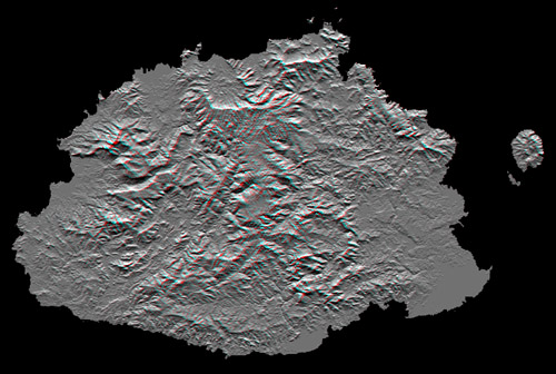
Anaglyph stereo image derived from Shuttle Radar Topography Mission data (NASA Jet Propulsion Laboratory, 2006).
The image above shows Viti Levu, the largest of the some 332 islands that comprise the Sovereign Democratic Republic of the Fiji Islands. Viti Levu’s area is 10,429 square kilometers (about 4000 square miles). Nakauvadra, the rugged mountain range running from north to south, has several peaks rising above 900 meters (about 3000 feet). Mount Tomanivi, in the upper center, is the highest peak at 1324 meters (4341 feet).
Learn more about the Shuttle Radar Topography Mission at Web sites published by NASA and USGS.
7.14. Bathymetry
The term bathymetry refers to the process and products of measuring the depth of water bodies. The U.S. Congress authorized the comprehensive mapping of the nation’s coasts in 1807, and directed that the task be carried out by the federal government’s first science agency, the Office of Coast Survey (OCS). That agency is now responsible for mapping some 3.4 million nautical square miles encompassed by the 12-mile territorial sea boundary, as well as the 200-mile Exclusive Economic Zone claimed by the U.S., a responsibility that entails regular revision of about 1,000 nautical charts. The coastal bathymetry data that appears on USGS topographic maps, like the one shown below, is typically compiled from OCS charts.
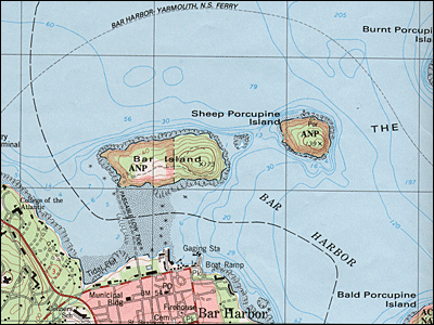
”Isobaths” (the technical term for lines of constant depth) shown on a USGS topographic map.
Early hydrographic surveys involved sampling water depths by casting overboard ropes weighted with lead and marked with depth intervals called marks and deeps. Such ropes were called leadlines for the weights that caused them to sink to the bottom. Measurements were called soundings. By the late 19th century, piano wire had replaced rope, making it possible to take soundings of thousands rather than just hundreds of fathoms (a fathom is six feet).

Seaman paying out a sounding line during a hydrographic survey of the East coast of the U.S. in 1916. (NOAA, 2007).
Echo sounders were introduced for deepwater surveys beginning in the 1920s. Sonar (SOund NAvigation and Ranging) technologies have revolutionized oceanography in the same way that aerial photography revolutionized topographic mapping. The seafloor topography revealed by sonar and related shipborne remote sensing techniques provided evidence that supported theories about seafloor spreading and plate tectonics.
Below is an artist’s conception of an oceanographic survey vessel operating two types of sonar instruments: multibeam and side scan sonar. On the left, a multibeam instrument mounted in the ship’s hull calculates ocean depths by measuring the time elapsed between the sound bursts it emits and the return of echoes from the seafloor. On the right, side scan sonar instruments are mounted on both sides of a submerged “towfish” tethered to the ship. Unlike multibeam, side scan sonar measures the strength of echoes, not their timing. Instead of depth data, therefore, side scanning produces images that resemble black-and-white photographs of the sea floor.
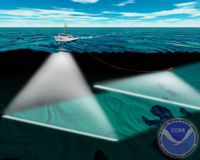
Multibeam and side scan sonar in use for bathymetric mapping. (NOAA, 2002).
A detailed report of the recent bathymetric survey of Crater Lake, Oregon, USA, is published by the USGS here.
7.15. Statistical Surfaces
Strategies used to represent terrain surfaces can be used for other kinds of surfaces as well. For example, one of my first projects here at Penn State was to work with a distinguished geographer, the late Peter Gould, who was studying the diffusion of the Acquired Immune Deficiency Syndrome (AIDS) virus in the United States. Dr. Gould had recently published the map below.

Oblique view of contour lines representing distribution of AIDS cases in the U.S. 1988. (Gould, 1989. © Association of American Geographers. All rights reserved. Reproduced here for educational purposes only).
Gould portrayed the distribution of disease in the same manner as another geographer might portray a terrain surface. The portrayal is faithful to Gould’s conception of the contagion as a continuous phenomenon. It was important to Gould that people understood that there was no location that did not have the potential to be visited by the epidemic. For both the AIDS surface and a terrain surface, a quantitative attribute (z) exists for every location (x,y). In general, when a continuous phenomenon is conceived as being analogous to the terrain surface, the conception is called a statistical surface.
7.16. Theme: Hydrography
The NSDI Framework Introduction and Reference (FGDC, 1997) envisions the hydrography theme in this way:
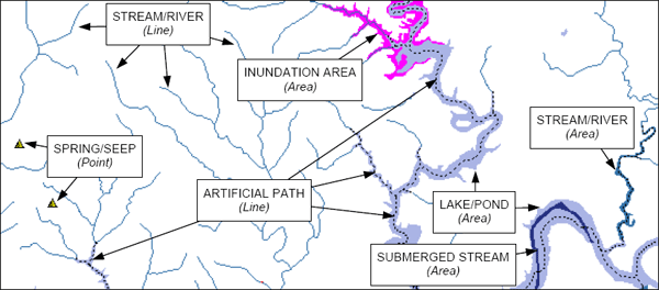
Framework hydrography data include surface water features such as lakes and ponds, streams and rivers, canals, oceans, and shorelines. Each of these features has the attributes of a name and feature identification code. Centerlines and polygons encode the positions of these features. For feature identification codes, many federal and state agencies use the Reach schedule developed by the U.S. Environmental Protection Agency (EPA).
Many hydrography data users need complete information about connectivity of the hydrography network and the direction in which the water flows encoded in the data. To meet these needs, additional elements representing flows of water and connections between features may be included in framework data (p. 20).
IDENTIFICATION
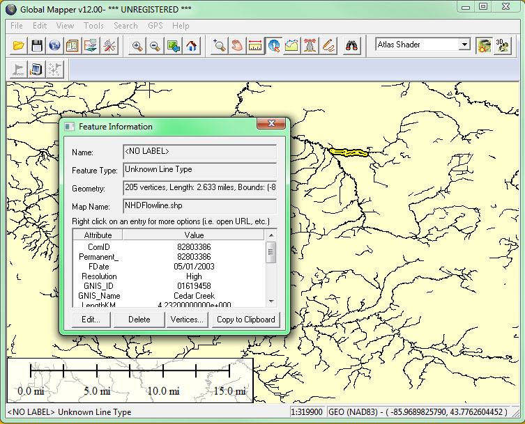
FGDC had the National Hydrography Dataset (NHD) in mind when they wrote this description. NHD combines the vector features ofDigital Line Graph (DLG) hydrography with the EPA’s Reach files. Reaches are segments of surface water that share similar hydrologic characteristics. Reaches are of three types: transport, coastline, and waterbody. DLG lines features represent the transport and coastline types; polygon features are used to represent waterbodies. Every reach segment in the NHD is assigned a unique reach code, along with a host of other hydrological attributes including stream flow direction (which is encoded in the digitizing order of nodes that make up each segment), network connectivity, and feature names, among others. Because the order of reach codes are sequential from reach to reach, point-source data (such as a pollutant spill) can be geocoded to the affected reach. Used in this way, reaches comprise alinear referencing system comparable to postal addresses along streets (USGS, 2002).
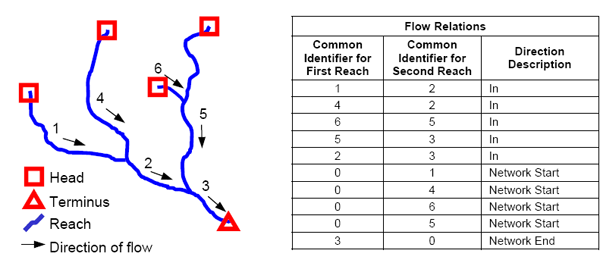
How flow attributes are associated with reaches in the National Hydrography Dataset (USGS, 2000).
NHD parses the U.S. surface drainage network into four hierarchical categories of units: 21 Regions, 222 Subregions, 352 Accounting units, and 2150 Cataloging units (also called Watersheds). Features can exist at multiple levels of the hierarchy, though they might not be represented in the same way. For example, while it might make the most sense to represent a given stream as a polygon features at the Watershed level, it may be more aptly represented as a line feature at the Region or Subregion level. NHD supports this by allowing multiple features to share the same reach codes. Another distinctive feature of NHD is artificial flowlines–centerline features that represent paths of water flow through polygon features such as standing water bodies. NHD is complex because it is designed to support sophisticated hydrologic modeling tasks, including point-source pollution modeling, flood potential, bridge construction, among others (Ralston, 2004).
How vector features are used to represent various types of reaches in the National Hydrography Dataset (USGS, 2000).
NHD are available at three levels of detail (scale): medium (1:100,000, which is available for the entire U.S.), high (1:24,000, production of which is underway, “according to the availability of matching resources from NHD partners” (USGS, 2002, p. 2), and local (larger scales such as 1:5,000), which “is being developed where partners and data exist” for select areas (USGS, 2006c; USGS, 2009; USGS 2013).
SPATIAL REFERENCE INFORMATION
NHD coordinates are decimal degrees referenced to the NAD 83 horizontal datum.
DISTRIBUTION
TRY THIS!
DOWNLOAD AND VIEW AN EXTRACT FROM THE NATIONAL HYDROGRAPHY DATASET
- From the NHD home page click the Get Data link and then follow the link to the NHD Viewer. (There is a Help button next to the viewer link.)
- Use the GIS tools, found above the map area, to pan to and zoom in on an area of interest. Then, click the Download Data button.
Choose a reference area from the pick list. (You could also chose the entire current map extent, but depending upon your zoom level that may be a huge dataset.)
Then click on the map to highlight a specific area of interest. A link to the available data sets will appear in the left hand pane under theSelection tab. (The All Results button will list the multiple areas you click on.) Follow the Download link of the area you are interested in. - In the USGS Available Data window that opens, selectHydrography from the Theme column, and choose a file format from the pick list in the Format column. I chose Shapefile format for my extract, because I know it is compatible with Global Mapper / dlgv32 Pro. If you were working in ArcGIS you could choose the File Geodatabase option. Ralston (2004, p.187) observes that NHD “is precisely the type of information that could benefit from an integrated data model in an object relational database.”
Click the Next button. - From the list of Hydrography Products check the box for what you wish to download. To be assured of getting the data in Shapefile format select a product referred to as a Dynamic Extract.
Click the Next button.
Go to the Cart pane on the right. (It may open automatically.)
Go to Checkout, supply your e-mail address, and submit your order via the Place Order button.
You will receive a message telling you that your order has been placed, and that will soon be followed by an e-mail regarding your order. About an hour and a half after I submitted my request I received a second e-mail containing a download link. - Extract the contents of the .zip file and view the Shapefile data set(s) in Global Mapper.
- Use the Identify pointer tool to reveal attributes of the reaches. In the example below I have highlighted a flowline associated with Cedar Creek in western Michigan.
7.17. Theme: Transportation
Transportation network data are valuable for all sorts of uses, including two we considered in Chapter 4: geocoding and routing. The Federal Geographic Data Committee (1997, p. 19) specified the following vector features and attributes for the transportation framework theme:
| Feature | Attributes |
|---|---|
| Roads | Centerlines, feature identification code (using linear referencing systems where available), functional class, name (including route numbers), and street address ranges |
| Trails | Centerlines, feature identification code (using linear referencing systems where available), name, and type |
| Railroads | Centerlines, feature identification code (using linear referencing systems where available), and type |
| Waterways | Centerlines, feature identification code (using linear referencing systems where available), and name |
| Airports and ports | Feature identification code and name |
| Bridges and tunnels | Feature identification code and name |
IDENTIFICATION
As part of the National Map initiative, USGS and partners are developing a comprehensive national database of vector transportation data. The transportation theme “includes best available data from Federal partners such as the Census Bureau and the Department of Transportation, State and local agencies” (USGS, 2007).
As envisioned by FGDC, centerlines are used to represent transportation routes. Like the lines painted down the middle of two-way streets, centerlines are 1-dimensional vector features that approximate the locations of roads, railroads, and navigable waterways. In this sense, road centerlines are analogous to the flowpaths encoded in the National Hydrologic Dataset (see previous page). Also like the NHD (and TIGER), road topology must be encoded to facilitate analysis of transportation networks.
To get a sense of the complexity of the features and attributes that comprise the transportation theme, see the Transportation Data Model(This is a 36″ x 48″ poster in a 5.2 Mb PDF file.) [The link to the Transportation Data Model poster recently became disconnected. Instead look at the model diagrams in the Part 7: Transportation Baseof the FGDC Geographic Framework Data Content Standard.]
In the U.S. at least, the best road centerline data is that produced by NAVTEQ and Tele Atlas, which license transportation data to routing sites like Google Maps and MapQuest, and to manufacturers of in-car GPS navigation systems. Because these data are proprietary, however, USGS must look elsewhere for data that can be made available for public use. TIGER/Line data produced by the Census Bureau will likely play an important role after the TIGER/MAF Modernization project is complete (see Chapter 4).
DISTRIBUTION
TRY THIS!
VIEW AND DOWNLOAD NATIONAL MAP TRANSPORTATION DATA
- Access the Viewer here.
- Expand the pane containing the layer options by clicking on Overlays at the upper-left.
- Under Base Data Layers, click on Transportation. You can expand the Transportation list and sub-select different layers.
- As you zoom in to larger map scales (using the slider bar at the upper-left of the map), additional transportation layers will become visible.
- If you wish to download an extract from the transportation database, click the Download Data button in the upper-right of the viewer interface and decide how you wish to extract the data. The Transportation data comes down in ESRI’s geodatabase format. Additional information regarding downloading data can be found via the Help button in the upper-right of the viewer interface.
7.18. Theme: Governmental Units
The FGDC framework also includes boundaries of governmental units, including:
- Nation
- States and statistically equivalent areas
- Counties and statistically equivalent areas
- Incorporated places and consolidated cities
- Functioning legal minor civil divisions
- Federal- or state-recognized American Indian reservations and trustlands
- Alaska native regional corporations
FGDC specifies that:
Each of these features includes the attributes of name and the applicable Federal Information Processing Standard (FIPS) code. Features boundaries include information about other features (such as road, railroads, or streams) with which the boundaries are associated and a description of the association (such as coincidence, offset, or corridor. (FGDC, 1997, p. 20-21)
IDENTIFICATION
The USGS National Map aspires to include a comprehensive database of boundary data. In addition to the entities outlined above, the National Map also lists congressional districts, school districts, and ZIP Code zones. Sources for these data include “Federal partners such as the U.S. Census Bureau, other Federal agencies, and State and local agencies.” (USGS, 2007).
To get a sense of the complexity of the features and attributes that comprise this theme, see the Governmental Units Data Model (This is a 36″ x 48″ poster in a 2.4 Mb PDF file.) [The link to the Governmental Units Data Model poster recently became disconnected. Instead look at the model diagrams in the Part 5: Governemntal unit and other geographic area boundaries of the FGDC Geographic Framework Data Content Standard.]
DISTRIBUTION
TRY THIS!
VIEW AND DOWNLOAD NATIONAL MAP GOVERNMENTAL UNITS DATA
- Access the Viewer here.
- Expand the pane containing the layer options by clicking on Overlays at the upper-left.
- Under Base Data Layers, click on Governmental Unit Boundaries. You can expand the this list and sub-select different boundary layers.
- As you zoom in to larger map scales (using the slider bar at the upper-left of the map), additional boundary layers will become visible.
- If you wish to download an extract from the Governmental Unit Boundaries database, click the Download Data button in the upper-right of the viewer interface and decide how you wish to extract the data. The Governmental Unit Boundaries data comes down in ESRI’s geodatabase format. Additional information regarding downloading data can be found via the Help button in the upper-right of the viewer interface.
7.19. Theme: Cadastral
FGDC (1997, p. 21) points out that:
Cadastral data represent the geographic extent of the past, current, and future rights and interests in real property. The spatial information necessary to describe the geographic extent and the rights and interests includes surveys, legal description reference systems, and parcel-by-parcel surveys and descriptions.
However, no one expects that legal descriptions and survey coordinates of private property boundaries (as depicted schematically in the portion of the plat map shown below) will be included in the USGS National Map any time soon. As discussed at the outset of Chapter 6, this is because local governments have authority for land title registration in the U.S., and most of these governments have neither the incentive nor the means to incorporate such data into a publicly-accessible national database.
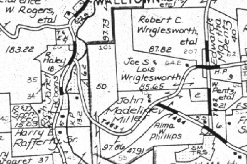
Plat maps are supplementary records that depict property parcel boundaries in graphic form. The geometric accuracy of plats is notoriously poor. The investment required to convert plat maps to properly georeferenced digital data is substantial. Many local governments have converted these records to digital form, or are in the process of doing so.
FGDC’s modest goal for the cadastal theme of the NSDI framework is to include:
…cadastral reference systems, such as the Public Land Survey System (PLSS) and similar systems not covered by the PLSS … and publicly administered parcels, such as military reservations, national forests, and state parks. (Ibid, p. 21)
FGDC’s Cadastral Data Content Standard is published here.
The colored areas on the map below show the extent of the United States Public Land Surveys, which commenced in 1784 and took nearly a century to complete (Muehrcke and Muehrcke, 1998). The purpose of the surveys was to partition “public land” into saleable parcels in order to raise revenues needed to retire war debt, and to promote settlement. A key feature of the system is its nomenclature, which provides concise, unique specifications of the location and extent of any parcel.
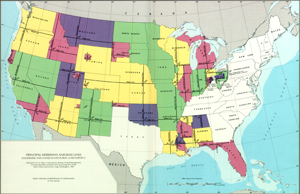
Extent of the U.S. Public Land Survey (Thompson, 1988).
Each Public Land Survey (shown in the colored areas above) commenced from an initial point at the precisely surveyed intersection of a base line and principal meridian. Surveyed lands were then partitioned into grids of townships each approximately six miles square.
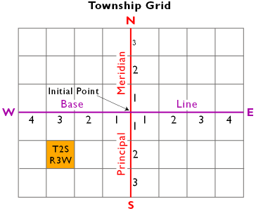
Townships are designated by their locations relative to the base line and principal meridian of a particular survey. For example, the township highlighted in gold above is the second township south of the baseline and the third township west of the principal meridian. The Public Land Survey designation for the highlighted township is “Township 2 South, Range 3 West.” Because of this nomenclature, the Public Land Survey System is also known as the “township and range system.” Township T2S, R3W is shown enlarged below.
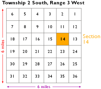
Townships are subdivided into grids of 36 sections. Each section covers approximately one square mile (640 acres). Notice the back-and-forth numbering scheme. Section 14, highlighted in gold above, is shown enlarged below.
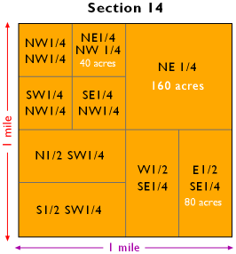
Inidividual property parcels are designated as shown above. For instance, the NE 1/4 of Section 14, Township 2 S, Range 3W, is a 160-acre parcel. Public Land Survey designations specify both the location of a parcel and its area.
The influence of the Public Land Survey grid is evident in the built environment of much of the American Midwest. As Mark Monmonier (1995, p. 114) observes:
The result [of the U.S. Public Land Survey] was an ‘authored landscape’ in which the survey grid had a marked effect on settlement patterns and the shapes of counties and smaller political units. In the typical Midwestern county, roads commonly following section lines, the rural population is dispersed rather than clustered, and the landscape has a pronounced checkerboard appearance.
For more information about the Public Land Survey System, see this article in the in the USGS’ National Atlas.
7.20. Summary
NSDI framework data represent “the most common data themes [that] users need” (FGDC, 1997, p. 3), including geodetic control, orthoimagery, elevation, hydrography, transportation, governmental unit boundaries, and cadastral reference information. Some themes, like transportation and governmental units, represent things that have well-defined edges. In this sense we can think of things like roads and political boundaries as discrete phenomena. The vector approach to geographic representation is well suited to digitizing discrete phenomena. Line features do a good job of representing roads, for example, and polygons are useful approximations of boundaries.
As you recall from Chapter 1, however, one of the distinguishing properties of the Earth’s surface is that it is continuous. Some phenomena distributed across the surface are continuous too. Terrain elevations, gravity, magnetic declination and surface air temperature can be measured practically everywhere. For many purposes, rasterdata are best suited to representing continuous phenomena.
An implication of continuity is that there is an infinite number of locations at which phenomena can be measured. It is not possible, obviously, to take an infinite number of measurements. Even if it were, the mass of data produced would not be usable. The solution, of course, is to collect a sample of measurements, and to estimate attribute values for locations that are left unmeasured. Chapter 7 also considers how missing elevations in a raster grid can be estimated from existing elevations, using a procedure called interpolation. The inverse distance weighted interpolation procedure relies upon another fundamental property of geographic data, spatial dependence.
The chapter concludes by investigating the characteristics and current status of the hydrography, transportation, governmental units, and cadastral themes. You had the opportunity to access, download, and open several of the data themes using viewers provided by USGS as part of its National Map initiative. In general, you should have found that although neither the NSDI or National Map visions have been fully realized, substantial elements of each is in place. Further progress depends on the American public’s continuing commitment to public data, and to the political will of our representatives in government.
QUIZ
Registered Penn State students should return now to the Chapter 7 folder in ANGEL (via the Resources menu to the left) to access the graded quiz for this chapter. This one counts. You may take graded quizzes only once.
The purpose of the quiz is to ensure that you have studied the text closely, that you have mastered the practice activities, and that you have fulfilled the chapter’s learning objectives. You are welcome to review the chapter during the quiz.
Once you have submitted the quiz and posted any questions you may have to either our discussion forums or chapter pages, you will have completed Chapter 7.
COMMENTS AND QUESTIONS
Registered students are welcome to post comments, questions, and replies to questions about the text. Particularly welcome are anecdotes that relate the chapter text to your personal or professional experience. In addition, there are discussion forums available in the ANGEL course management system for comments and questions about topics that you may not wish to share with the whole world.
To post a comment, scroll down to the text box under “Post new comment” and begin typing in the text box, or you can choose to reply to an existing thread. When you are finished typing, click on either the “Preview” or “Save” button (Save will actually submit your comment). Once your comment is posted, you will be able to edit or delete it as needed. In addition, you will be able to reply to other posts at any time.
Note: the first few words of each comment become its “title” in the thread.
7.21. Bibliography
Federal Geographic Data Committee (1997). Framework introduction and guide. Washington DC: Federal Geographic Data Committee.
Eischeid, J. D., Baker, C. B., Karl, R. R., Diaz, H. F. (1995). The quality control of long-term climatological data using objective data analysis. Journal of Applied Meteorology, 34, 27-88.
Gould, P. (1989). Geographic dimensions of the AIDS epidemic.Professional Geographer, 41:1, 71-77.
Maune, D. F. (Ed.) (2007). Digital elevation model technologies and applications: The DEM users manual, 2nd edition. Bethesda, MD: American Society for Photogrammetric Engineering and Remote Sensing.
Monmonier, M. S. (1982). Drawing the line: tales of maps and cartocontroversy. New York, NY: Henry Holt.
Muehrcke, P. C. and Muehrcke, J. O. (1998) Map use, 4th Ed. Madison, WI: JP Publications.
National Aeronautics and Space Administration, Jet Propulsion Laboratory (2006). Shuttle radar topography mission. Retrieved May 10, 2006, from http://www.jpl.nasa.gov/srtm
Goddard Space Flight Center, National Aeronautics and Space Administration (n.d.). Greenland’s receding ice. Retrieved Feburary 26, 2008, from http://svs.gsfc.nasa.gov/stories/greenland/
National Geophysical Data Center (2010). ETOPO1 global gridded 1 arc-minute database. Retrieved March 2, 2010, fromhttp://www.ngdc.noaa.gov/mgg/global/global.html
National Oceanic and Atmospheric Administration, National Climatic Data Center (n. d.). Merged land-ocean seasonal temperature anomalies. Retrieved August 18, 1999, fromwww.ncdc.noaa.giv/onlineprod/landocean/seasonal/form.html(expired)
National Oceanic and Atmospheric Administration (2002). Side scan and multibeam sonar. Retrieved February 18, 2008, fromhttp://www.nauticalcharts.noaa.gov/hsd/hydrog.htm
National Oceanic and Atmospheric Administration (2007). NOAA History. Retrieved February 27, 2008, fromhttp://www.history.noaa.gov/
Rabenhorst, T. D. and McDermott, P. D. (1989). Applied cartography: source materials for mapmaking. Columbus, OH: Merrill.
Raitz, E. (1948). General cartography. New York, NY: McGraw-Hill.
Ralston, B. A. (2004). GIS and public data. Clifton Park NY: Delmar Learning.
Thompson, M. M. (1988) Maps for america, 3rd Ed. Reston, VA: United States Geological Survey.
United States Geological Survey (1987) Digital elevation models. Data users guide 5. Reston, VA: USGS.
United States Geological Survey (1999) The National Hydrography Dataset. Fact Sheet 106-99. Reston, VA: USGS. Retrieved February 19, 2008 from http://erg.usgs.gov/isb/pubs/factsheets/fs10699.html
United States Geological Survey (2000) The National Hydrography Dataset: Concepts and Contents. Reston, VA: USGS. Retrieved February 19, 2008 fromhttp://nhd.usgs.gov/chapter1/chp1_data_users_guide.pdf
United States Geological Survey (2002) The National Map – Hydrography. Fact Sheet 060-02. Reston, VA: USGS. Retrieved February 19, 2008 fromhttp://erg.usgs.gov/isb/pubs/factsheets/fs06002.html Retrieved September 22, 2013 from http://pubs.er.usgs.gov/publication/fs06002
United States Geological Survey (2006a) Digital Line Graphs (DLG). Reston, VA: USGS. Retrieved February 18, 2008 fromedc.usgs.gov/products/map/dlg.html (In 2010 the site becamehttp://eros.usgs.gov/#/Find_Data/Products_and_Data_Available/DLGs)
United States Geological Survey (2006b) GTOPO30. Retrieved February 27, 2008 fromedc.usgs.gov/products/elevation/gtopo30/gtopo30.html since moved to http://www1.gsi.go.jp/geowww/globalmap-gsi/gtopo30/gtopo30.html
United States Geological Survey (2006c) National Hydrography Dataset (NHD) – High-resolution (Metadata). Reston, VA: USGS. Retrieved February 19, 2008 fromnhdgeo.usgs.gov/metadata/nhd_high.htm
United States Geological Survey (2007). Vector data theme development of The National Map. Retrieved 24 February 2008 frombpgeo.cr.usgs.gov/model/ (expired or moved)
United States Geological Survey (2009) The National Map – Hydrography Dataset. Reston, VA: USGS. Retrieved September 22, 2013 from http://pubs.usgs.gov/fs/2009/3054/pdf/FS2009-3054.pdf
United States Geological Survey (2013) National Hydrography Dataset (NHD) – Get NDH Data. Reston, VA: USGS. Retrieved September 22, 2013 from http://nhd.usgs.gov/data.html