
5: Land Surveying and GPS
- Page ID
- 8171

Land Surveying and GPS
David DiBiase
5.1. Overview
As you recall from Chapter 1, geographic data represent spatial locations and non-spatial attributes measured at certain times. We defined “feature” as a set of positions that specifies the location and extent of an entity. Positions, then, are a fundamental element of geographic data. Like the letters that make up these words, positions are the building blocks from which features are constructed. A property boundary, for example, is made up of a set of positions connected by line segments.
In theory, a single position is a “0-dimensional” feature: an infinitesimally small point from which 1-dimensional, 2-dimensional, and 3-dimensional features (lines, areas, and volumes) are formed. In practice, positions occupy 2- or 3-dimensional areas as a result of the limited resolution of measurement technologies and the limited precision of location coordinates. Resolution and precision are two aspects of data quality. This chapter explores the technologies and procedures used to produce positional data, and the factors that determine its quality.
Objectives
Students who successfully complete Chapter 5 should be able to:
- Identify and define the key aspects of data quality, including resolution, precision, and accuracy;
- List and explain the procedures land surveyors use to produce positional data, including traversing, triangulation, and trilateration;
- Calculate plane coordinates by open traverse;
- Calculate elevations by leveling;
- Explain how radio signals broadcast by Global Positioning System satellites are used to calculate positions on the surface of the Earth;
- State the kinds and magnitude of error associated with uncorrected GPS positioning; and
- Identify and explain methods used to improve the accuracy of GPS positioning.
Comments and Questions
Registered students are welcome to post comments, questions, and replies to questions about the text. Particularly welcome are anecdotes that relate the chapter text to your personal or professional experience. In addition, there are discussion forums available in the ANGEL course management system for comments and questions about topics that you may not wish to share with the whole world.
To post a comment, scroll down to the text box under “Post new comment” and begin typing in the text box, or you can choose to reply to an existing thread. When you are finished typing, click on either the “Preview” or “Save” button (Save will actually submit your comment). Once your comment is posted, you will be able to edit or delete it as needed. In addition, you will be able to reply to other posts at any time.
Note: the first few words of each comment become its “title” in the thread.
5.2. Checklist
The following checklist is for Penn State students who are registered for classes in which this text, and associated quizzes and projects in the ANGEL course management system, have been assigned. You may find it useful to print this page out first so that you can follow along with the directions.
| Step | Activity | Access/Directions |
|---|---|---|
| 1 | Read Chapter 5 | This is the second page of the Chapter. Click on the links at the bottom of the page to continue or to return to the previous page, or to go to the top of the chapter. You can also navigate the text via the links in the GEOG 482 menu on the left. |
| 2 | Submit five practice quizzesincluding:
Practice quizzes are not graded and may be submitted more than once. | Go to ANGEL > [your course section] > Lessons tab > Chapter 5 folder > [quiz] |
| 3 | Perform “Try this” activitiesincluding:
“Try this” activities are not graded. | Instructions are provided for each activity. |
| 4 | Submit theChapter 5 Graded Quiz | ANGEL > [your course section] > Lessons tab > Chapter 5 folder > Chapter 5 Graded Quiz. See the Calendar tab in ANGEL for due dates. |
| 5 | Read comments and questionsposted by fellow students. Add comments and questions of your own, if any. | Comments and questions may be posted on any page of the text, or in a Chapter-specific discussion forum in ANGEL. |
5.3. Geospatial Data Quality
Quality is a characteristic of comparable things that allows us to decide that one thing is better than another. In the context of geographic data, the ultimate standard of quality is the degree to which a data set is fit for use in a particular application. That standard is called validity. The standard varies from one application to another. In general, however, the key criteria are how much error is present in a data set, and how much error is acceptable.
Some degree of error is always present in all three components of geographic data: features, attributes, and time. Perfect data would fully describe the location, extent, and characteristics of phenomena exactly as they occur at every moment. Like the proverbial 1:1 scale map, however, perfect data would be too large, and too detailed to be of any practical use. Not to mention impossibly expensive to create in the first place!
5.4. Error and Uncertainty
Positions are the products of measurements. All measurements contain some degree of error. Errors are introduced in the original act of measuring locations on the Earth surface. Errors are also introduced when second- and third-generation data is produced, say, by scanning or digitizing a paper map.
In general, there are three sources of error in measurement: human beings, the environment in which they work, and the measurement instruments they use.
Human errors include mistakes, such as reading an instrument incorrectly, and judgments. Judgment becomes a factor when the phenomenon that is being measured is not directly observable (like an aquifer), or has ambiguous boundaries (like a soil unit).
Environmental characteristics, such as variations in temperature, gravity, and magnetic declination, also result in measurement errors.
Instrument errors follow from the fact that space is continuous. There is no limit to how precisely a position can be specified. Measurements, however, can be only so precise. No matter what instrument, there is always a limit to how small a difference is detectable. That limit is calledresolution.
The diagram below shows the same position (the point in the center of the bullseye) measured by two instruments. The two grid patterns represent the smallest objects that can be detected by the instruments. The pattern at left represents a higher-resolution instrument.
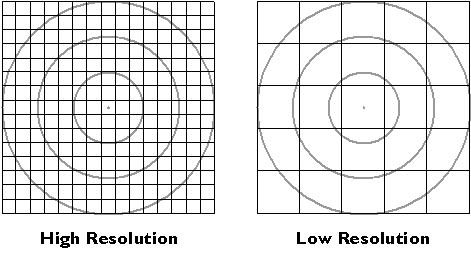
Resolution.
The resolution of an instrument affects the precision of measurements taken with it. In the illustration below, the measurement at left, which was taken with the higher-resolution instrument, is more precise than the measurement at right. In digital form, the more precise measurement would be represented with additional decimal places. For example, a position specified with the UTM coordinates 500,000. meters East and 5,000,000. meters North is actually an area 1 meter square. A more precise specification would be 500,000.001 meters East and 5,000,000.001 meters North, which locates the position within an area 1 millimeter square. You can think of the area as a zone of uncertainty within which, somewhere, the theoretically infinitesimal point location exists.Uncertainty is inherent in geospatial data.
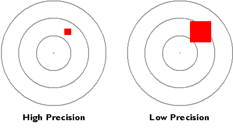
The precision of a single measurement.
Precision takes on a slightly different meaning when it is used to refer to a number of repeated measurements. In the illustration below, there is less variance among the nine measurements at left than there is among the nine measurements at right. The set of measurements at left is said to be more precise.
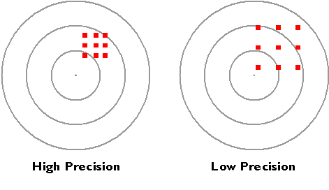
The precision of multiple measurements.
Hopefully you have noticed that resolution and precision are independent from accuracy. As shown below, accuracy simply means how closely a measurement corresponds to an actual value.
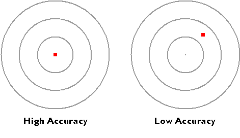
Accuracy.
I mentioned the U.S. Geological Survey’s National Map Accuracy Standard in Chapter 2. In regard to topographic maps, the Standard warrants that 90 percent of well-defined points tested will be within a certain tolerance of their actual positions. Another way to specify the accuracy of an entire spatial database is to calculate the average difference between many measured positions and actual positions. The statistic is called the root mean square error (RMSE) of a data set.
5.5. Systematic vs. Random Errors
The diagram below illustrates the distinction between systematic andrandom errors. Systematic errors tend to be consistent in magnitude and/or direction. If the magnitude and direction of the error is known, accuracy can be improved by additive or proportional corrections.Additive correction involves adding or subtracting a constant adjustment factor to each measurement; proportional correction involves multiplying the measurement(s) by a constant.
Unlike systematic errors, random errors vary in magnitude and direction. It is possible to calculate the average of a set of measured positions, however, and that average is likely to be more accurate than most of the measurements.
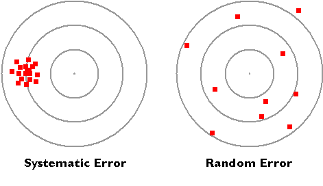
Systematic and random errors.
In the sections that follow we compare the accuracy and sources of error of two important positioning technologies: land surveying and the Global Positioning System.
5.6. Survey Control
Geographic positions are specified relative to a fixed reference. Positions on the globe, for instance, may be specified in terms of angles relative to the center of the Earth, the equator, and the prime meridian. Positions in plane coordinate grids are specified as distances from the origin of the coordinate system. Elevations are expressed as distances above or below a vertical datum such as mean sea level, or an ellipsoid such as GRS 80 or WGS 84, or a geoid.
Land surveyors measure horizontal positions in geographic or plane coordinate systems relative to previously surveyed positions called control points. In the U.S., the National Geodetic Survey (NGS) maintains aNational Spatial Reference System (NSRS) that consists of approximately 300,000 horizontal and 600,000 vertical control stations (Doyle,1994). Coordinates associated with horizontal control points are referenced to NAD 83; elevations are relative to NAVD 88. In a Chapter 2 activity you may have retrieved one of the datasheets that NGS maintains for every NSRS control point, along with more than a million other points submitted by professional surveyors.
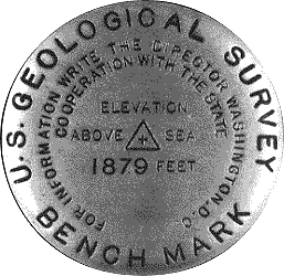
Benchmark used to mark a vertical control point. (Thompson, 1988).
In 1988 NGS established four orders of control point accuracy, which are outlined in the table below. The minimum accuracy for each order is expressed in relation to the horizontal distance separating two control points of the same order. For example, if you start at a control point of order AA and measure a 500 km distance, the length of the line should be accurate to within 3 mm base error, plus or minus 5 mm line length error (500,000,000 mm × 0.01 parts per million).
| Order | Survey activities | Maximum base error(95% confidence limit) | Maximum Line-length dependent error(95% confidence limit) |
|---|---|---|---|
| AA | Global-regional dynamics; deformation measurements | 3 mm | 1:100,000,000 (0.01 ppm) |
| A | NSRS primary networks | 5 mm | 1:10,000,000 (0.1 ppm) |
| B | NSRS secondary networks; high-precision engineering surveys | 8 mm | 1:1,000,000 (1 ppm) |
| C | NSRS terrestrial; dependent control surveys for mapping, land information, property, and engineering requirements | 1st: 1.0 cm 2nd-I: 2.0 cm 2nd-II: 3.0 cm 3rd: 5.0 cm | 1st: 1:100,000 2nd-I: 1:50,000 2nd-II: 1:20,000 3rd: 1:10,000 |
Control network accuracy standards used for U.S. National Spatial Reference System (Federal Geodetic Control Committee, 1988).
Doyle (1994) points out that horizontal and vertical reference systems coincide by less than ten percent. This is because
….horizontal stations were often located on high mountains or hilltops to decrease the need to construct observation towers usually required to provide line-of-sight for triangulation, traverse and trilateration measurements. Vertical control points however, were established by the technique of spirit leveling which is more suited to being conducted along gradual slopes such as roads and railways that seldom scale mountain tops. (Doyle, 2002, p. 1)
You might wonder how a control network gets started. If positions are measured relative to other positions, what is the first position measured relative to? The answer is: the stars. Before reliable timepieces were available, astronomers were able to determine longitude only by careful observation of recurring celestial events, such as eclipses of the moons of Jupiter. Nowadays geodesists produce extremely precise positional data by analyzing radio waves emitted by distant stars. Once a control network is established, however, surveyors produce positions using instruments that measure angles and distances between locations on the Earth’s surface.
6.7. Measuring Angles
Angles can be measured with a magnetic compass, of course. Unfortunately, the Earth’s magnetic field does not yield the most reliable measurements. The magnetic poles are not aligned with the planet’s axis of rotation (an effect called magnetic declination), and they tend to change location over time. Local magnetic anomalies caused by magnetized rocks in the Earth’s crust and other geomagnetic fields make matters worse.
For these reasons land surveyors rely on transits (or their more modern equivalents, called theodolites) to measure angles. A transit consists of a telescope for siting distant target objects, two measurement wheels that work like protractors for reading horizontal and vertical angles, and bubble levels to ensure that the angles are true. A theodolite is essentially the same instrument, except that some mechanical parts are replaced with electronics.
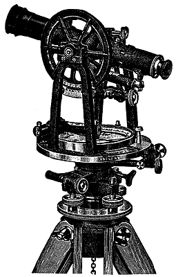
Transit. (Raisz, 1948). Used by permission.
Surveyors express angles in several ways. When specifying directions, as is done in the preparation of a property survey, angles may be specified as bearings or azimuths. A bearing is an angle less than 90° within a quadrant defined by the cardinal directions. An azimuth is an angle between 0° and 360° measured clockwise from North. “South 45° East” and “135°” are the same direction expressed as a bearing and as an azimuth. An interior angle, by contrast, is an angle measured between two lines of sight, or between two legs of a traverse (described later in this chapter).
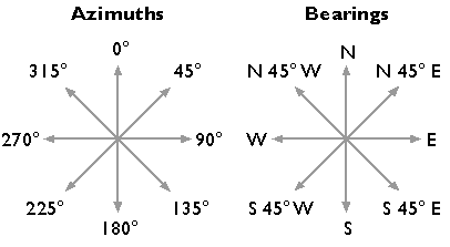
Azimuths and bearings.
In the U.S., professional organizations like the American Congress on Surveying and Mapping, the American Land Title Association, the National Society of Professional Surveyors, and others, recommend minimum accuracy standards for angle and distance measurements. For example, as Steve Henderson (personal communication, Fall 2000, updated July 2010) points out, the Alabama Society of Professional Land Surveyors recommends that errors in angle measurements in “commercial/high risk” surveys be no greater than 15 seconds times the square root of the number of angles measured.
To achieve this level of accuracy, surveyors must overcome errors caused by faulty instrument calibration; wind, temperature, and soft ground; and human errors, including misplacing the instrument and misreading the measurement wheels. In practice, surveyors produce accurate data by taking repeated measurements and averaging the results.
8. Measuring Distances
To measure distances, land surveyors once used 100-foot long metal tapes that are graduated in hundredths of a foot. (This is the technique I learned as a student in a surveying class at the University of Wisconsin in the early 1980s. The picture shown below is slightly earlier.) Distances along slopes are measured in short horizontal segments. Skilled surveyors can achieve accuracies of up to one part in 10,000 (1 centimeter error for every 100 meters distance). Sources of error include flaws in the tape itself, such as kinks; variations in tape length due to extremes in temperature; and human errors such as inconsistent pull, allowing the tape to stray from the horizontal plane, and incorrect readings.
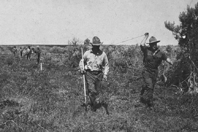
Surveying team measuring a baseline distance with a metal (Invar) tape. (Hodgson, 1916).
Since the 1980s, electronic distance measurement (EDM) devices have allowed surveyors to measure distances more accurately and more efficiently than they can with tapes. To measure the horizontal distance between two points, one surveyor uses an EDM instrument to shoot an energy wave toward a reflector held by the second surveyor. The EDM records the elapsed time between the wave’s emission and its return from the reflector. It then calculates distance as a function of the elapsed time. Typical short-range EDMs can be used to measure distances as great as 5 kilometers at accuracies up to one part in 20,000, twice as accurate as taping.
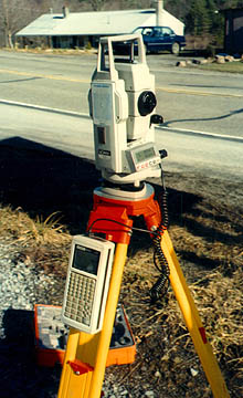
Total station.
Instruments called total stations combine electronic distance measurement and the angle measuring capabilities of theodolites in one unit. Next we consider how these instruments are used to measure horizontal positions in relation to established control networks.
5.9. Horizontal Positions
Surveyors have developed distinct methods, based on separate control networks, for measuring horizontal and vertical positions. In this context, a horizontal position is the location of a point relative to two axes: the equator and the prime meridian on the globe, or x and y axes in a plane coordinate system. Control points tie coordinate systems to actual locations on the ground; they are the physical manifestations of horizontal datums. In the following pages we review two techniques that surveyors use to create and extend control networks (triangulation and trilateration) and two other techniques used to measure positions relative to control points (open and closed traverses).
5.10. Traverse
Surveyors typically measure positions in series. Starting at control points, they measure angles and distances to new locations, and use trigonometry to calculate positions in a plane coordinate system. Measuring a series of positions in this way is known as “running a traverse.” A traverse that begins and ends at different locations is called an open traverse.
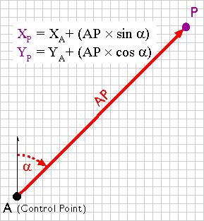
An open traverse. (Adapted from Robinson, et al., 1995)
For example, say the UTM coordinates of point A in the illustration above are 500,000.00 E and 5,000,000.00 N. The distance between points A and P, measured with a steel tape or an EDM, is 2,828.40 meters. The azimuth of the line AP, measured with a transit or theodolite, is 45º. Using these two measurements, the UTM coordinates of point P can be calculated as follows:
XP = 500,000.00 + (2,828.40 × sin 45) = 501,999.98
YP = 5,000,000.00 + (2,828.40 × cos 45°) = 5,001,999.98
A traverse that begins and ends at the same point, or at two different but known points, is called a closed traverse. Measurement errors in a closed traverse can be quantified by summing the interior angles of the polygon formed by the traverse. The accuracy of a single angle measurement cannot be known, but since the sum of the interior angles of a polygon is always (n-2) × 180, it’s possible to evaluate the traverse as a whole, and to distribute the accumulated errors among all the interior angles.
Errors produced in an open traverse, one that does not end where it started, cannot be assessed or corrected. The only way to assess the accuracy of an open traverse is to measure distances and angles repeatedly, forward and backward, and to average the results of calculations. Because repeated measurements are costly, other surveying techniques that enable surveyors to calculate and account for measurement error are preferred over open traverses for most applications.
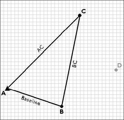
5.11. Triangulation
Closed traverses yield adequate accuracy for property boundary surveys, provided that an established control point is nearby. Surveyors conductcontrol surveys to extend and densify horizontal control networks. Before survey-grade satellite positioning was available, the most common technique for conducting control surveys was triangulation.
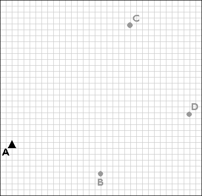
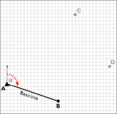
The purpose of a control survey is to establish new horizontal control points (B, C, and D) based upon an existing control point (A).
Using a total station equipped with an electronic distance measurement device, the control survey team commences by measuring the azimuthalpha, and the baseline distance AB. These two measurements enable the survey team to calculate position B as in an open traverse. Before geodetic-grade GPS became available, the accuracy of the calculated position B may have been evaluated by astronomical observation.
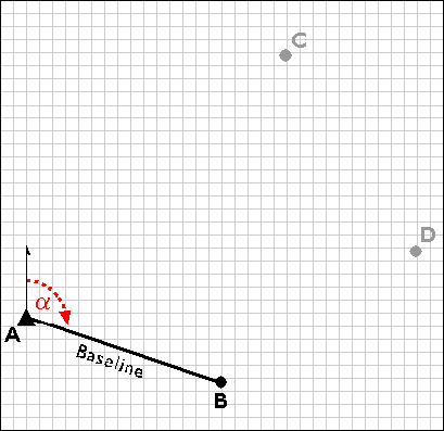
Establishing a second control point (B) in a triangulation network.
The surveyors next measure the interior angles CAB, ABC, and BCA at point A, B, and C. Knowing the interior angles and the baseline length, the trigonometric “law of sines” can then be used to calculate the lengths of any other side. Knowing these dimensions, surveyors can fix the position of point C.
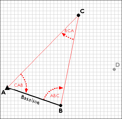
Establishing the position of point C by triangulation.
Having measured three interior angles and the length of one side of triangle ABC, the control survey team can calculate the length of side BC. This calculated length then serves as a baseline for triangle BDC. Triangulation is thus used to extend control networks, point by point and triangle by triangle.
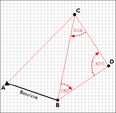
Extending the triangulation network.
5.12. Trilateration
Trilateration is an alternative to triangulation that relies upon distance measurements only. Electronic distance measurement technologies make trilateration a cost-effective positioning technique for control surveys. Not only is it used by land surveyors, trilateration is also used to determine location coordinates with Global Positioning System satellites and receivers.

Trilateration is used to extend control networks by establishing new control points (B, C, and D) based upon existing control points (A).
Trilateration networks commence the same way as triangulation nets. If only one existing control point is available, a second point (B) is established by open traverse. Using a total station equipped with an electronic distance measurement device, the survey team measures the azimuth α and baseline distance AB. The total station operator may set up her instrument over point A, while her assistant holds a reflector mounted on a shoulder-high pole as steadily as he can over point B. Depending on the requirements of the control survey, the accuracy of the calculated position B may be confirmed by astronomical observation.
Establishing a second control point (B) in a trilateration network.
Next, the survey team uses the electronic distance measurement feature of the total station to measure the distances AC and BC. Both forward and backward measurements are taken. After the measurements are reduced from slope distances to horizontal distances, the law of cosines can be employed to calculate interior angles, and the coordinates of position C can be fixed. The accuracy of the fix is then checked by plotting triangle ABC and evaluating the error of closure.
Measuring the distances AC and BC.
Next, the trilateration network is extended by measuring the distances CD and BD, and fixing point D in a plane coordinate system.
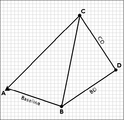
Fixing control point D by trilateration.
TRY THIS!
USE TRILATERATION TO DETERMINE A CONTROL POINT LOCATION
Trilateration is a technique land surveyors use to calculate an undetermined position in a plane coordinate system by measuring distances from two known positions. As you will see later in this chapter, trilateration is also the technique that GPS receivers use to calculate their positions on the Earth’s surface, relative to the positions of three or more satellite transmitters. The purpose of this exercise is to make sure you understand how trilateration works. (Estimated time to complete: 5 minutes.)
Note: You will need to have the Adobe Flash player installed in order to complete this exercise. If you do not already have the Flash player, you can download it for free from Adobe.
- Display a coordinate system grid: In this exercise, you will interact with a coordinate system grid. First, display the coordinate system grid in a separate window so that you can interact with it while you read these instructions. Arrange the coordinate system grid window and this window so that you can easily view both. You may need to make this window more narrow. Two control points, A and B, are plotted in the coordinate system grid. A survey crew has measured distances from the control points to another point, point C, whose coordinates are unknown. Your job is to fix the position of point C. You will find point C at the intersection of two circles centered on control points A and B, where the radii of the two circles equals the measured distances from the control points to point C.
- Plot the distance from control point A to point C: On the coordinate system grid, click on control point A to display the data entry form. (You’ll need to click on the actual point, not the “A”.) The form consists of a text field in which you can type in a distance, and a button that plots a circle centered on point A. The radius of the circle will be the distance you specify. According to the surveyors’ measurements, the distance between control point A and point C is 9400 feet. Enter that distance now and click Plot to plot the circle. [View result of Step 2]
- Plot the distance from control point B to point C: The measured distance from point B to point C is 7000 feet. Click on point B (on the actual point, not the “B”), enter that distance and plot a circle. [View result of Step 3]
- Plot point C: Now click within the coordinate grid to reveal the position of point C. You may have to hunt for it, but you should know where to look based on the intersection of the circles. [View result of Step 4]
- Extend the control network further: Now continue extending the control network by plotting a fourth point, point D, in the coordinate system grid. First plot new circles at points A and C. The measured distance from point A to point D is 9600 feet. The measured distance from point C to point D is 8000 feet. (You may wish to set the radius of the circle centered upon point B to 0.) Finally, click in the coordinate system grid to plot point D. [View result of Step 5]
Once you have finished viewing the grid, close the popup window.
PRACTICE QUIZ
Registered Penn State students should return now to the Chapter 5 folder in ANGEL (via the Resources menu to the left) to take a self-assessment quiz about Horizontal Positions. You may take practice quizzes as many times as you wish. They are not scored and do not affect your grade in any way.
5.13. Vertical Positions
A vertical position is the height of a point relative to some reference surface, such as mean sea level, a geoid, or an ellipsoid. The roughly 600,000 vertical control points in the U.S. National Spatial Reference System (NSRS) are referenced to the North American Vertical Datum of 1988 (NAVD 88). Surveyors created the National Geodetic Vertical Datum of 1929 (NGVD 29, the predecessor to NAVD 88), by calculating the average height of the sea at all stages of the tide at 26 tidal stations over 19 years. Then they extended the control network inland using a surveying technique called leveling. Leveling is still a cost-effective way to produce elevation data with sub-meter accuracy.
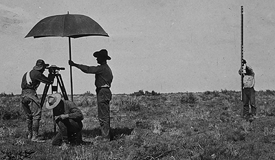
A leveling crew at work in 1916. (Hodgson, 1916).
The illustration above shows a leveling crew at work. The fellow under the umbrella is peering through the telescope of a leveling instrument. Before taking any measurements, the surveyor made sure that the telescope was positioned midway between a known elevation point and the target point. Once the instrument was properly leveled, he focused the telescope crosshairs on a height marking on the rod held by the fellow on the right side of the picture. The chap down on one knee is noting in a field book the height measurement called out by the telescope operator.
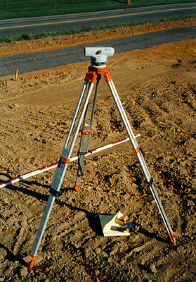
A level used for determining elevations.
Leveling is still a cost-effective way to produce elevation data with sub-meter accuracy. A modern leveling instrument is shown in the photograph above. The diagram below illustrates the technique called differential leveling.
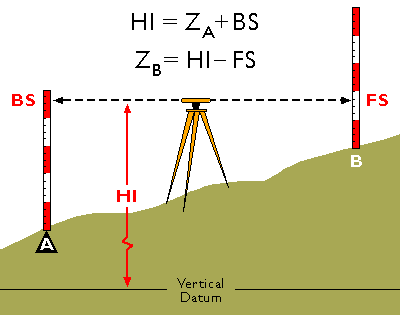
Differential leveling. (Adapted from Wolf & Brinker, 1994)
The diagram above illustrates differential leveling. A leveling instrument is positioned midway between a point at which the ground elevation is known (point A) and a point whose elevation is to be measured (B). The height of the instrument above the datum elevation is HI. The surveyor first reads a backsight measurement (BS) off of a leveling rod held by his trusty assistant over the benchmark at A. The height of the instrument can be calculated as the sum of the known elevation at the benchmark (ZA) and the backsight height (BS). The assistant then moves the rod to point B. The surveyor rotates the telescope 180°, then reads a foresight (FS) off the rod at B. The elevation at B (ZB) can then be calculated as the difference between the height of the instrument (HI) and the foresight height (FS).
Former student Henry Whitbeck (personal communication, Fall 2000) points out that surveyors also use total stations to measure vertical angles and distances between fixed points (prisms mounted upon tripods at fixed heights), then calculate elevations by trigonometric leveling.
HEIGHTS
Surveyors use the term height as a synonym for elevation. There are several different ways to measure heights. A properly-oriented level defines a line parallel to the geoid surface at that point (Van Sickle, 2001).An elevation above the geoid is called an orthometric height.However, GPS receivers cannot produce orthometric heights directly. Instead, GPS produces heights relative to the WGS 84 ellipsoid.Elevations produced with GPS are therefore called ellipsoidal (or geodetic) heights.
PRACTICE QUIZ
Registered Penn State students should return now to the Chapter 5 folder in ANGEL (via the Resources menu to the left) to take a self-assessment quiz about Vertical Positions. You may take practice quizzes as many times as you wish. They are not scored and do not affect your grade in any way.
5.14. Global Positioning System
Positioning signals broadcast from three Global Positioning System satellites are received at a location on Earth. (U.S. Federal Aviation Administration, 2007b)
The Global Positioning System (GPS) employs trilateration to calculate the coordinates of positions at or near the Earth’s surface.Trilateration refers to the trigonometric law by which the interior angles of a triangle can be determined if the lengths of all three triangle sides are known. GPS extends this principle to three dimensions.
A GPS receiver can fix its latitude and longitude by calculating its distance from three or more Earth-orbiting satellites, whose positions in space and time are known. If four or more satellites are within the receiver’s “horizon,” the receiver can also calculate its elevation, and even its velocity. The U.S. Department of Defense created the Global Positioning System as an aid to navigation. Since it was declared fully operational in 1994, GPS positioning has been used for everything from tracking delivery vehicles, to tracking the minute movements of the tectonic plates that make up the Earth’s crust, to tracking the movements of human beings. In addition to the so-called user segment made up of the GPS receivers and people who use them to measure positions, the system consists of two other components: a space segment and a control segment. It took about $10 billion to build over 16 years.
Russia maintains a similar positioning satellite system called GLONASS. Member nations of the European Union are in the process of deploying a comparable system of their own, called Galileo. The first experimental GIOVE-A satellite began transmitting Galileo signals in January 2006. The goal of the Galileo project is a constellation of 30 navigation satellites by 2020. If the engineers and politicians succeed in making Galileo, GLONASS, and the U.S. Global Positioning System interoperable, as currently seems likely, the result will be a Global Navigation Satellite System (GNSS) that provides more than twice the signal-in-space resource that is available with GPS alone. The Chinese began work on their own system, called Beidou, in 2000. At the end of 2011 they had ten satellites in orbit, serving just China, with the goal being a global system of 35 satellites by 2020.
In this section you will learn to:
- Explain how radio signals broadcast by Global Positioning System satellites are used to calculate positions on the surface of the Earth; and
- Describe the functions of the space, control, and user segments of the Global Positioning System.
5.15. Space Segment
The space segment of the Global Positioning System currently consists of approximately 30 active and spare NAVSTAR satellites (new satellites are launched periodically, and old ones are decommissioned). “NAVSTAR” stands for “NAVigation System with Timing And Ranging.” Each satellite circles the Earth every 12 hours in sidereal time along one of six orbital “planes” at an altitude of 20,200 km (about 12,500 miles). The satellites broadcast signals used by GPS receivers on the ground to measure positions. The satellites are arrayed such that at least four are “in view” everywhere on or near the Earth’s surface at all times, with typically up to eight and potentially 12 “in view” at any given time.
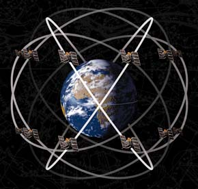
The constellation of GPS satellites. Illustration © Smithsonian Institution, 1988. Used by Permission.
TRY THIS!
The U.S. Coast Guard’s Navigation Center publishes status reports on the GPS satellite constellation. Its report of August 17, 2010, for example, listed 31 satellites, five to six in each of the six orbits planes (A-F), and one scheduled outage, on August 19, 2010. You can look up the current status of the constellation here.
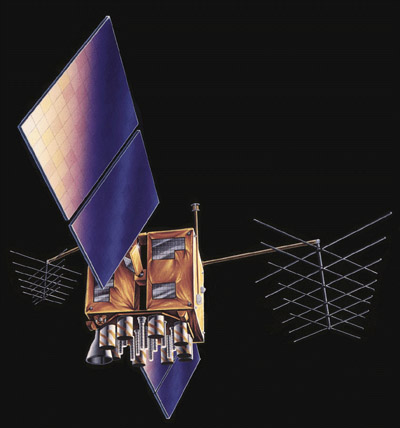
Artist’s rendition of a NAVSTAR satellite (NAVSTAR GPS Joint Program Office, n.d.).
TRY THIS!
Scientific programmers at the U.S. National Aeronautics and Space Administration (NASA) have created an interactive, three-dimensional model of the Earth and the orbits of the more than 500 man-made satellites that surround it. The model is a Java applet called J-Track 3D Satellite Tracking. Your browser must have Java enabled to view the applet. Instructions at the site describe how you can zoom in and out, and drag to rotate the model. To view orbits of particular satellites, choose Select from the Satellite menu. The Block IIA and R series are the most current generation of NAVSTAR satellites.
5.16. Control Segment
The control segment of the Global Positioning System is a network of ground stations that monitors the shape and velocity of the satellites’ orbits. The accuracy of GPS data depends on knowing the positions of the satellites at all times. The orbits of the satellites are sometimes disturbed by the interplay of the gravitational forces of the Earth and Moon.
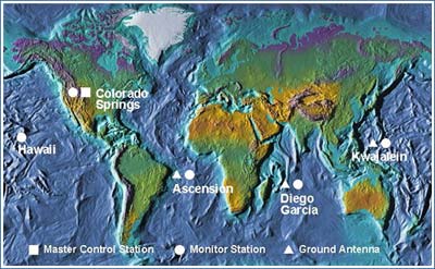
The control segment of the Global Positioning System (U.S. Federal Aviation Administration, 2007b).
Monitor Stations are very precise GPS receivers installed at known locations. They record discrepancies between known and calculated positions caused by slight variations in satellite orbits. Data describing the orbits are produced at the Master Control Station at Colorado Springs, uploaded to the satellites, and finally broadcast as part of the GPS positioning signal. GPS receivers use this satellite Navigation Message data to adjust the positions they measure.
If necessary, the Master Control Center can modify satellite orbits by commands transmitted via the control segment’s ground antennas.
5.17. User Segment
The U.S. Federal Aviation Administration (FAA) estimated in 2006 that some 500,000 GPS receivers are in use for many applications, including surveying, transportation, precision farming, geophysics, and recreation, not to mention military navigation. This was before in-car GPS navigation gadgets emerged as one of the most popular consumer electronic gifts during the 2007 holiday season in North America.
Basic consumer-grade GPS receivers, like the rather old-fashioned one shown below, consist of a radio receiver and internal antenna, a digital clock, some sort of graphic and push-button user interface, a computer chip to perform calculations, memory to store waypoints, jacks to connect an external antenna or download data to a computer, and flashlight batteries for power. The radio receiver in the unit shown below includes 12 channels to receive signal from multiple satellites simultaneously.
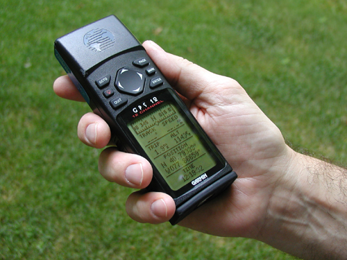
Recreation-grade GPS receiver, circa 1998.
NAVSTAR Block II satellites broadcast at two frequencies, 1575.42 MHz (L1) and 1227.6 MHz (L2). (For sake of comparison, FM radio stations broadcast in the band of 88 to 108 MHz.) Only L1 was intended for civilian use. Single-frequency receivers produce horizontal coordinates at an accuracy of about three to seven meters (or about 10 to 20 feet) at a cost of about $100. Some units allow users to improve accuracy by filtering out errors identified by nearby stationary receivers, a post-process called “differential correction.” $300-500 single-frequency units that can also receive corrected L1 signals from the U.S. Federal Aviation Administration’s Wide Area Augmentation System (WAAS) network of ground stations and satellites can perform differential correction in “real-time.” Differentially-corrected coordinates produced by single-frequency receivers can be as accurate as one to three meters (about 3 to 10 feet).
The signal broadcast at the L2 frequency is encrypted for military use only. Clever GPS receiver makers soon figured out, however, how to make dual-frequency models that can measure slight differences in arrival times of the two signals (these are called “carrier phase differential” receivers). Such differences can be used to exploit the L2 frequency to improve accuracy without decoding the encrypted military signal. Survey-grade carrier-phase receivers able to perform real-time kinematic (RTK) differential correction, can produce horizontal coordinates at sub-meter accuracy at a cost of $1000 to $2000. No wonder GPS has replaced electro-optical instruments for many land surveying tasks.
Meanwhile, a new generation of NAVSTAR satellites (the Block IIR-M series) will add a civilian signal at the L2 frequency that will enable substantially improved GPS positioning.
5.18. Satellite Ranging
GPS receivers calculate distances to satellites as a function of the amount of time it takes for satellites’ signals to reach the ground. To make such a calculation, the receiver must be able to tell precisely when the signal was transmitted, and when it was received. The satellites are equipped with extremely accurate atomic clocks, so the timing of transmissions is always known. Receivers contain cheaper clocks, which tend to be sources of measurement error. The signals broadcast by satellites, called “pseudo-random codes,” are accompanied by the broadcast ephemeris data that describes the shapes of satellite orbits.
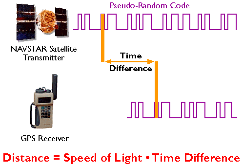
GPS receivers calculate distance as a function of the difference in time of broadcast and reception of a GPS signal. (Adapted from Hurn, 1989).
The GPS constellation is configured so that a minimum of four satellites is always “in view” everywhere on Earth. If only one satellite signal was available to a receiver, the set of possible positions would include the entire range sphere surrounding the satellite.
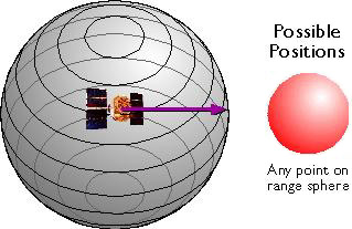
Set of possible positions of a GPS receiver relative to a single GPS satellite. (Adapted from Hurn, 1993).
If two satellites are available, a receiver can tell that its position is somewhere along a circle formed by the intersection of two spherical ranges.
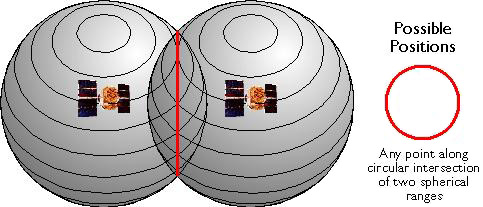
Set of possible positions of a GPS receiver relative to two GPS satellites. (Adapted from Hurn, 1993).
If distances from three satellites are known, the receiver’s position must be one of two points at the intersection of three spherical ranges. GPS receivers are usually smart enough to choose the location nearest to the Earth’s surface. At a minimum, three satellites are required for a two-dimensional (horizontal) fix. Four ranges are needed for a three-dimensional fix (horizontal and vertical).
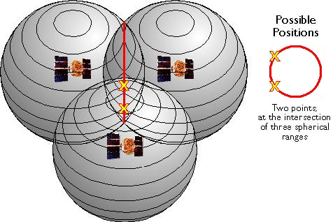
Set of possible positions of a GPS receiver relative to three GPS satellites. (Adapted from Hurn, 1993).
Satellite ranging is similar in concept to the plane surveying methodtrilateration, by which horizontal positions are calculated as a function of distances from known locations. The GPS satellite constellation is in effect an orbiting control network.
TRY THIS!
Trimble has a tutorial “designed to give you a good basic understanding of the principles behind GPS without loading you down with too much technical detail”. Check it out at http://www.trimble.com/gps_tutorial/. Click “Why GPS?” to get started.
PRACTICE QUIZ
Registered Penn State students should return now to the Chapter 5 folder in ANGEL (via the Resources menu to the left) to take a self-assessment quiz about GPS Components. You may take practice quizzes as many times as you wish. They are not scored and do not affect your grade in any way.
5.19. GPS Error Sources
A thought experiment (Wormley, 2004): Attach your GPS receiver to a tripod. Turn it on and record its position every ten minutes for 24 hours. Next day, plot the 144 coordinates your receiver calculated. What do you suppose the plot would look like?
Do you imagine a cloud of points scattered around the actual location? That’s a reasonable expectation. Now, imagine drawing a circle or ellipse that encompasses about 95 percent of the points. What would the radius of that circle or ellipse be? (In other words, what is your receiver’s positioning error?)
The answer depends in part on your receiver. If you used a hundred-dollar receiver, the radius of the circle you drew might be as much as ten meters to capture 95 percent of the points. If you used a WAAS-enabled, single frequency receiver that cost a few hundred dollars, your error ellipse might shrink to one to three meters or so. But if you had spent a few thousand dollars on a dual frequency, survey-grade receiver, your error circle radius might be as small as a centimeter or less. In general, GPS users get what they pay for.
As the market for GPS positioning grows, receivers are becoming cheaper. Still, there are lots of mapping applications for which it’s not practical to use a survey-grade unit. For example, if your assignment was to GPS 1,000 manholes for your municipality, you probably wouldn’t want to set up and calibrate a survey-grade receiver 1,000 times. How, then, can you minimize errors associated with mapping-grade receivers? A sensible start is to understand the sources of GPS error.
In this section you will learn to:
- State the kinds and magnitude of error and uncertainty associated with uncorrected GPS positioning; and
- Use a PDOP chart to determine the optimal times for GPS positioning at a given location and date.
Note: My primary source for the material in this section is Jan Van Sickle’s text GPS for Land Surveyors, 2nd Ed. If you want a readable and much more detailed treatment of this material, I recommend Jan’s book. See the bibliography at the end of this chapter for more information about this and other resources.
5.20. User Equivalent Range Errors
“UERE” is the umbrella term for all of the error sources below, which are presented in descending order of their contributions to the total error budget.
- Satellite clock: GPS receivers calculate their distances from satellites as a function of the difference in time between when a signal is transmitted by a satellite and when it is received on the ground. The atomic clocks on board NAVSTAR satellites are extremely accurate. They do tend to stray up to one millisecond of standard GPS time (which is calibrated to, but not identical to, Coordinated Universal Time). The monitoring stations that make up the GPS “Control Segment” calculate the amount of clock drift associated with each satellite. GPS receivers that are able to make use of the clock correction data that accompanies GPS signals can reduce clock error significantly.
- Upper atmosphere (ionosphere): Space is nearly a vacuum, but the atmosphere isn’t. GPS signals are delayed and deflected as they pass through the ionosphere, the outermost layers of the atmosphere that extend from approximately 50 to 1,000 km above the Earth’s surface. Signals transmitted by satellites close to the horizon take a longer route through the ionosphere than signals from satellites overhead, and are thus subject to greater interference. The ionosphere’s density varies by latitude, by season, and by time of day, in response to the Sun’s ultraviolet radiation, solar storms and maximums, and the stratification of the ionosphere itself. The GPS Control Segment is able to model ionospheric biases, however. Monitoring stations transmit corrections to the NAVSTAR satellites, which then broadcast the corrections along with the GPS signal. Such corrections eliminate only about three-quarters of the bias, however, leaving the ionosphere the second largest contributor to the GPS error budget.
- Receiver clock: GPS receivers are equipped with quartz crystal clocks that are less stable than the atomic clocks used in NAVSTAR satellites. Receiver clock error can be eliminated, however, by comparing times of arrival of signals from two satellites (whose transmission times are known exactly).
- Satellite orbit: GPS receivers calculate coordinates relative to the known locations of satellites in space. Knowing where satellites are at any given moment involves knowing the shapes of their orbits as well as their velocities. The gravitational attractions of the Earth, Sun, and Moon all complicate the shapes of satellite orbits. The GPS Control Segment monitors satellite locations at all times, calculates orbit eccentricities, and compiles these deviations in documents called ephemerides. An ephemeris is compiled for each satellite and broadcast with the satellite signal. GPS receivers that are able to process ephemerides can compensate for some orbital errors.
- Lower atmosphere: (troposphere, tropopause, and stratosphere) The three lower layers of atmosphere encapsulate the Earth from surface to an altitude of about 50 km. The lower atmosphere delays GPS signals, adding slightly to the calculated distances between satellites and receivers. Signals from satellites close to the horizon are delayed the most, since they pass through more atmosphere than signals from satellites overhead.
- Multipath: Ideally, GPS signals travel from satellites through the atmosphere directly to GPS receivers. In reality, GPS receivers must discriminate between signals received directly from satellites and other signals that have been reflected from surrounding objects, such as buildings, trees, and even the ground. Some, but not all, reflected signals are identified automatically and rejected. Antennas are designed to minimize interference from signals reflected from below, but signals reflected from above are more difficult to eliminate. One technique for minimizing multipath errors is to track only those satellites that are at least 15° above the horizon, a threshold called the “mask angle.”
Douglas Welsh (personal communication, Winter 2001), an Oil and Gas Inspector Supervisor with Pennsylvania’s Department of Environmental Protection, wrote about the challenges associated with GPS positioning in our neck of the woods: “…in many parts of Pennsylvania the horizon is the limiting factor. In a city with tall buildings and the deep valleys of some parts of Pennsylvania it is hard to find a time of day when the constellation will have four satellites in view for any amount of time. In the forests with tall hardwoods, multipath is so prevalent that I would doubt the accuracy of any spot unless a reading was taken multiple times.” Van Sickle (2005) points out, however, that GPS modernization efforts and the GNSS may well ameliorate such gaps.
Have you had similar experiences with GPS? If so, please post a comment to this page .
5.21. Dilution of Precision
The arrangement of satellites in the sky also affects the accuracy of GPS positioning. The ideal arrangement (of the minimum four satellites) is one satellite directly overhead, three others equally spaced near the horizon (above the mask angle). Imagine a vast umbrella that encompasses most of the sky, where the satellites form the tip and the ends of the umbrella spines.
GPS coordinates calculated when satellites are clustered close together in the sky suffer from dilution of precision (DOP), a factor that multiplies the uncertainty associated with User Equivalent Range Errors (UERE – errors associated with satellite and receiver clocks, the atmosphere, satellite orbits, and the environmental conditions that lead to multipath errors). The DOP associated with an ideal arrangement of the satellite constellation equals approximately 1, which does not magnify UERE. According to Van Sickle (2001), the lowest DOP encountered in practice is about 2, which doubles the uncertainty associated with UERE.
GPS receivers report several components of DOP, including Horizontal Dilution of Precision (HDOP) and Vertical Dilution of Precision (VDOP). The combination of these two components of the three-dimensional position is called PDOP – position dilution of precision. A key element of GPS mission planning is to identify the time of day when PDOP is minimized. Since satellite orbits are known, PDOP can be predicted for a given time and location. Various software products allow you to determine when conditions are best for GPS work.
MGIS student Jason Setzer (Winter 2006) offers the following illustrative anecdote:
I have had a chance to use GPS survey technology for gathering ground control data in my region and the biggest challenge is often the PDOP (position dilution of precision) issue. The problem in my mountainous area is the way the terrain really occludes the receiver from accessing enough satellite signals.
During one survey in Colorado Springs I encountered a pretty extreme example of this. Geographically, Colorado Springs is nestled right against the Rocky Mountain front ranges, with 14,000 foot Pike’s Peak just west of the city. My GPS unit was easily able to ‘see’ five, six or even seven satellites while I was on the eastern half of the city. However, the further west I traveled, I began to see progressively less of the constellation, to the point where my receiver was only able to find one or two satellites. If a 180 degree horizon-to-horizon view of the sky is ideal, then in certain places I could see maybe 110 degrees.
There was no real work around, other than patience. I was able to adjust my survey points enough to maximize my view of the sky. From there it was just a matter of time… Each GPS bird has an orbit time of around twelve hours, so in a couple of instances I had to wait up to two hours at a particular location for enough of them to become visible. My GPS unit automatically calculates PDOP and displays the number of available satellites. So the PDOP value was never as low as I would have liked, but it did drop enough to finally be within acceptable limits. Next time I might send a vendor out for such a project!
TRY THIS!
Trimble, a leading manufacturer of GPS receivers, offers GPS mission planning software for free downloads. This activity will introduce you to the capabilities of the software, and will prepare you to answer questions about GPS mission planning later.
(The mission planning software is a Windows application (.exe). Mac users, as well as Windows users, see beneath the numbered steps.)
- Visit the Trimble website
- Download the Trimble planning software, install it on your computer (note where it is installing its Common Files), and launch the application.
- Install an almanac: In the Almanac menu, move your cursor to Importand in the submenu, choose Almanac | navigate to the folder where the Common Files were installed | select almanac.alm and click the Openbutton | click OK.
(If your Windows operating system is installed on your C-drive, then the path name to the almanac.alm file probably looks like this, with or without the “(x86)”:
C:Program Files (x86)Common FilesTrimblePlanning) - Choose File | Station… Choose a location at which you might wish to plan a GPS mission.
- Choose Satellite | Information to explore the characteristics of active GPS, GLONASS, and WAAS satellites.
- Choose Graphs | DOP | DOP – position to see how combined HDOP and VDOP vary throughout a selected 24-hour period at your selected location. Can you determine the best and worst times of day for GPS work?
While Trimble still makes available for free the planning software that you used above, they are not including access to an up to date almanac (information about currently available satellites). You may have noticed that the almanac you loaded was from 2010.
However, if you go here you will find an interactive interface that gives you access to a more current version of the same functionality as the planning app used above.
PRACTICE QUIZ
Registered Penn State students should return now to the Chapter 5 folder in ANGEL (via the Resources menu to the left) to take a self-assessment quiz about GPS Error Sources. You may take practice quizzes as many times as you wish. They are not scored and do not affect your grade in any way.
5.22. GPS Error Correction
A variety of factors, including the clocks in satellites and receivers, the atmosphere, satellite orbits, and reflective surfaces near the receiver, degrade the quality of GPS coordinates. The arrangement of satellites in the sky can make matters worse (a condition called dilution of precision). A variety of techniques have been developed to filter out positioning errors. Random errors can be partially overcome by simply averaging repeated fixes at the same location, although this is often not a very efficient solution. Systematic errors can be compensated for by modeling the phenomenon that causes the error and predicting the amount of offset. Some errors, like multipath errors caused when GPS signals are reflected from roads, buildings, and trees, vary in magnitude and direction from place to place. Other factors, including clocks, the atmosphere, and orbit eccentricities, tend to produce similar errors over large areas of the Earth’s surface at the same time. Errors of this kind can be corrected using a collection of techniques called differential correction.
In this section you will learn to:
- Explain the concept of differential correction and other methods used to improve the accuracy of GPS positioning; and
- Perform differential correction using data and services of the U.S. National Geodetic Survey.
5.23. Differential Correction
Differential correction is a class of techniques for improving the accuracy of GPS positioning by comparing measurements taken by two or more receivers. Here’s how it works:
The locations of two GPS receivers–one stationary, one mobile–are illustrated below. The stationary receiver (or “base station”) continuously records its fixed position over a control point. The difference between the base station’s actual location and its calculated location is a measure of the positioning error affecting that receiver at that location at each given moment. In this example, the base station is located about 25 kilometers from the mobile receiver (or “rover”). The operator of the mobile receiver moves from place to place. The operator might be recording addresses for an E-911 database, or trees damaged by gypsy moth infestations, or street lights maintained by a public works department
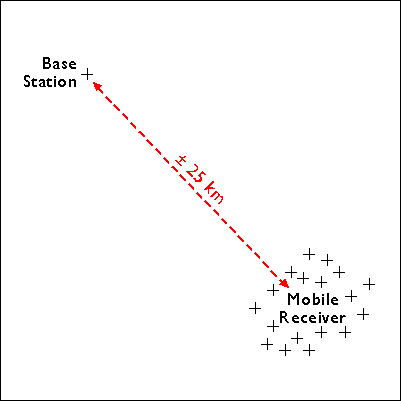
A GPS base station is fixed over a control point, while about 25 km away, a mobile GPS receiver is used to measure a series of positions.
The illustration below shows positions calculated at the same instant (3:01 pm) by the base station (left) and the mobile receiver (right).
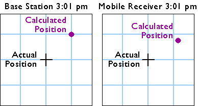
Actual and calculated positions of a base station and mobile receiver.
The base station calculates the correction needed to eliminate the error in the position calculated at that moment from GPS signals. The correction is later applied to the position calculated by the mobile receiver at the same instant. The corrected position is not perfectly accurate because the kinds and magnitudes of errors affecting the two receivers are not identical, and because of the low frequency of the GPS timing code.
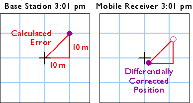
Error correction calculated at the base station is applied to the position calculated by the mobile receiver.
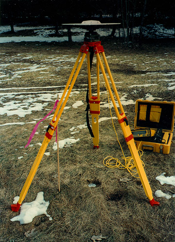
GPS base station used for differential correction. Notice that the antenna is located directly above a control point monument.
5.24. Real-Time Differential Correction
For differential correction to work, fixes recorded by the mobile receiver must be synchronized with fixes recorded by the base station (or stations). You can provide your own base station, or use correction signals produced from reference stations maintained by the U.S. Federal Aviation Administration, the U.S. Coast Guard, or other public agencies or private subscription services. Given the necessary equipment and available signals, synchronization can take place immediately (“real-time”) or after the fact (“post-processing”). First let’s consider real-time differential.
WAAS-enabled receivers are an inexpensive example of real-time differential correction. “WAAS” stands for Wide Area Augmentation System, a collection of about 25 base stations set up to improve GPS positioning at U.S. airport runways to the point that GPS can be used to help land airplanes (U.S. Federal Aviation Administration, 2007c). WAAS base stations transmit their measurements to a master station, where corrections are calculated and then uplinked to two geosynchronous satellites (19 are planned). The WAAS satellite then broadcasts differentially-corrected signals at the same frequency as GPS signals. WAAS signals compensate for positioning errors measured at WAAS base stations, as well as clock error corrections and regional estimates of upper-atmosphere errors (Yeazel, 2003). WAAS-enabled receivers devote one or two channels to WAAS signals, and are able to process the WAAS corrections. The WAAS network was designed to provide approximately 7-meter accuracy uniformly throughout its U.S. service area.
DGPS: The U.S. Coast Guard has developed a similar system, called theDifferential Global Positioning Service. The DGPS network includes some 80 broadcast sites, each of which includes a survey-grade base station and a “radiobeacon” transmitter that broadcasts correction signals at 285-325 kHz (just below the AM radio band). DGPS-capable GPS receivers include a connection to a radio receiver that can tune in to one or more selected “beacons.” Designed for navigation at sea near U.S. coasts, DGPS provides accuracies no worse than 10 meters. Stephanie Brown (personal communication, Fall 2003) reported that where she works in Georgia, “with a good satellite constellation overhead, [DGPS accuracy] is typically 4.5 to 8 feet.”
Survey-grade real-time differential correction can be achieved using a technique called real-time kinematic (RTK) GPS. According to surveyor Laverne Hanley (personal communication, Fall 2000), “real-time kinematic requires a radio frequency link between a base station and the rover. I have achieved better than centimeter accuracy this way, although the instrumentation is touchy and requires great skill on the part of the operator. Several times I found that I had great GPS geometry, but had lost my link to the base station. The opposite has also happened, where I wanted to record positions and had a radio link back to the base station, but the GPS geometry was bad.”
5.25. Post-Processed Differential Correction
Kinematic positioning can deliver accuracies of 1 part in 100,000 to 1 part in 750,000 with relatively brief observations of only one to two minutes each. For applications that require accuracies of 1 part in 1,000,000 or higher, including control surveys and measurements of movements of the Earth’s tectonic plates, static positioning is required (Van Sickle, 2001). In static GPS positioning, two or more receivers measure their positions from fixed locations over periods of 30 minutes to two hours. The receivers may be positioned up to 300 km apart. Onlydual frequency, carrier phase differential receivers capable of measuring the differences in time of arrival of the civilian GPS signal (L1) and the encrypted military signal (L2) are suitable for such high-accuracy static positioning.
CORS and OPUS: The U.S. National Geodetic Survey (NGS) maintains an Online Positioning User Service (OPUS) that enables surveyors to differentially-correct static GPS measurements acquired with a single dual frequency carrier phase differential receiver after they return from the field. Users upload measurements in a standard Receiver INdependent EXchange format (RINEX) to NGS computers, which perform differential corrections by referring to three selected base stations selected from a network of continuously operating reference stations. NGS oversees two CORS networks; one consisting of its 600 base stations of its own, another a cooperative of public and private agencies that agree to share their base station data and to maintain base stations to NGS specifications.
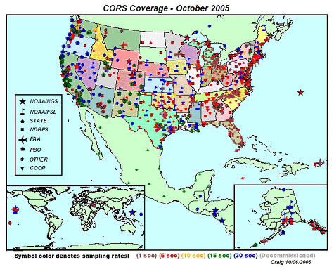
The Continuously Operating Reference Station network (CORS) (Snay, 2005)
The map above shows distribution of the combined national and cooperative CORS networks. Notice that station symbols are colored to denote the sampling rate at which base station data are stored. After 30 days, all stations are required to store base station data only in 30 second increments. This policy limits the utility of OPUS corrections to static positioning (although the accuracy of longer kinematic observations can also be improved). Mindful of the fact that the demand for static GPS is steadily declining, NGS’ future plans include streaming CORS base station data for real-time use in kinematic positioning.
TRY THIS!
This optional activity (contributed by Chris Piburn of CompassData Inc.) will guide you through the process of differentially-correcting static GPS measurements using the NGS’ Online Positioning User Service (OPUS), which refers to the Continuously Operating Reference Station network (CORS).
The context is a CompassData project that involved a carrier phase differential GPS survey in a remote study area in Alaska. The objective was to survey a set of nine ground control points (GCPs) that would later be used to orthorectify a client’s satellite imagery. So remote is this area that no NGS control point was available at the time the project was carried out. The alternative was to establish a base station for the project and to fix its position precisely with reference to CORS stations in operation elsewhere in Alaska.
The project team flew by helicopter to a hilltop located centrally within the study area. With some difficulty they hammered an 18 inch #5 rebar into the rocky soil to serve as a control monument. After setting up a GPS base station receiver over the rebar, they flew off to begin data collection with their rover receiver. Thanks to favorable weather, Chris and his team collected the nine required photo-identifiable GCPs on the first day. The centrally-located base station allowed the team to minimize distances between the base and the rover, which meant they could minimize the time required to fix each GCP. At the end of the day, the team had produced five hours of GPS data at the base station and nine fifteen-minute occupations at the GCPs
As you might expect, the raw GPS data were not sufficiently accurate to meet project requirements. (The various sources of random and systematic errors that contribute to the uncertainty of GPS data are considered elsewhere in this chapter.) In particular, the monument hammered into the hilltop was unsuitable for use as a control point because the uncertainty associated with its position was too great. The project team’s first step in removing positioning errors was to post-process the data using baseline processing software, which adjusts computed baseline distances (between the base station and the nine GCPs) by comparing the phase of the GPS carrier wave as it arrived simultaneously at both the base station and the rover. The next step was to fix the position of the base station precisely in relation to CORS stations operating elsewhere in Alaska.
The following steps will guide you through the process of submitting the five hours of dual frequency base station data to the U.S. National Geodetic Survey’s Online Positioning User Service (OPUS), and interpreting the results. (For information about OPUS, go here)
1. Download the GPS data file. The compressed RINEX format file is approximately 6 Mb in size and will take about 1 minute to download via high speed DSL or cable, or about 15 minutes via 56 Kbps modem. If you can’t download this file, contact me right away so we can help you resolve the problem.
- WILD282u.zip (5.8 Mb)
GPS receivers produce data in their manufacturers’ proprietary formats. NGS requires that the GPS data be converted to the “Receiver INdependent EXchange” format (RINEX) for compatibility with OPUS. Most software packages that come with the GPS units themselves have a built in utility to convert their GPS data to RINEX format. NGS itself uses free conversion software provided by a non-profit, government-sponsored consortium called UNAVCO.
2. Examine the RINEX file.
- Extract the RINEX file “WILD282u.05O” from its ZIP archive.
- Open “WILD282u.05O” with Microsoft Notepad or WordPad. (WordPad does a better job of preserving columns of text in this case. Set the word wrap to off.) Or, use another text editor. (In any open text editor window, in the File > Open dialog, make sure “Files of type:” is set to “All files” so that the target file is listed.)
The RINEX Observation file contains all the information about the signals that CompassData’s base station receiver tracked during the Alaska survey. Explaining all the contents of the file is well beyond the scope of this activity. For now, note the lines that disclose the antenna type, approximate position of the antenna, and antenna height. You’ll report these parameters to OPUS in the next step.
3. Submit GPS data to OPUS
- Point your browser to the OPUS home page and enter the information needed in order to “Upload your data file.”
- (OPUS step 1) Click the Browse button to call up a File Upload window. Navigate to and upload the RINEX file you downloaded earlier. To streamline your submission, choose the compressed archive “WILD282u.zip”.
- (OPUS step 2) Select the antenna type. Refer to the line labeled “ANT # / TYPE” in the RINEX file you opened in your text editor. You should find the antenna type “TPSHIPER_PLUS”. Choose this type from the pull-down list.
- (OPUS step 3) Enter the height of the antenna above the monument. Refer to the line labeled “ANTENNA: DELTA H/E/N” in the RINEX file you opened in your text editor. The first value on that line, “1.0854″, is H, in meters. (See the OPUS website for more information about antenna height.)
- (OPUS step 4) Enter the email address to which you wish your results to be returned.
- (OPUS step 5) Options. OPUS allows users to specify a State Plane Coordinate system zone, to select or exclude particular CORS reference stations, to request standard or extended output, and to establish a user profile for use with future jobs. For this activity, no changes to the default settings are needed.
- (OPUS step 6) Click the “Upload to STATIC” button to submit the data for differential correction in relation to three CORS reference stations. Depending on how many requests are in NGS’ queue, results may be returned in minutes or hours. When this activity was tested, the queue included only one request (see window below, which appears after requests successfully submitted) and results were returned in just a few minutes, but in the past it has taken up to 10 minutes.
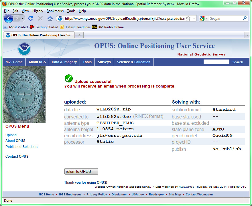
Upload results report, Online Positioning User Service, U.S. National Geodetic Survey.
When you receive your OPUS solution by return email, you will want to discover the magnitude of differential correction that OPUS calculated. To do this you’ll need to determine (a) the uncorrected position originally calculated by the base station, (b) the corrected position calculated by OPUS, and (c) the mark-to-mark distance between the original and corrected positions. In addition to the original RINEX file you downloaded earlier, you’ll need the OPUS solution and two free software utilities provided by NGS. Links to these utilities are listed below.
4. Determine the position of the base station receiver prior to differential correction.
- Refer to the RINEX file “WILD282u.05O” you opened in your text editor. The ninth line of the RINEX file lists the position of the base station receiver in Earth-Centered Earth-Fixed X, Y, Z coordinates. This is a three-dimensional Cartesian coordinate system whose origin is the Earth’s center of mass (like the NAD 83 datum).-2389892.2740 -1608765.8567 5672855.7386 APPROX POSITION XYZ
NGS provides a conversion utility to transform these X, Y, Z values to more familiar latitude and longitude coordinates and ellipsoidal heights.
- Go to NGS’ XYZ to GEODETIC conversion.
- Enter the X, Y, Z coordinates found in the RINEX file. Your result should be:
- Latitude = 63°13’53.74280″ N
- Longitude = 146°03’12.12710″ W
- Height = 1349.2248 m
5. Determine the corrected position of the base station receiver. The OPUS solution you receive by email reports corrected coordinates in Earth-Centered Earth-Fixed X, Y, Z, as geographic coordinates, and as UTM and State Plane coordinates. Look for the latitude and longitude coordinates and ellipsoidal height that are specified relative to the NAD 83 datum. They should be very close to:
- Latitude = 63°13’53.73892″ N
- Longitude = 146°03’11.98942″ W
- Height = 1348.756 m
6. Calculate the difference between the original and corrected base station positions. NGS provides another software utility to calculate the three-dimensional distance between two positions. Unlike the previous XYZ to GEODETIC converter, however, the “invers3d.exe” is a program you download to your computer.
- Download “invers3d.exe”
- Double-click on the file name to run the program, and choose thegeodetic coordinates option.
- Paying close attention to the required formats, enter the uncorrected latitude, longitude, and ellipsoidal heights you calculated in step 4 above.
- Next, choose the geodetic coordinates option again, enter the corrected coordinates and height you calculated in step 5.
- Among the results, look for the calculated “mark-to-mark distance.” This is the magnitude of the OPUS correction.
PRACTICE QUIZ
Registered Penn State students should return now to the Chapter 5 folder in ANGEL (via the Resources menu to the left) to take a self-assessment quiz about GPS Error Correction. You may take practice quizzes as many times as you wish. They are not scored and do not affect your grade in any way.
5.26. Summary
Positions are a fundamental element of geographic data. Sets of positions form features, as the letters on this page form words. Positions are produced by acts of measurement, which are susceptible to human, environmental, and instrument errors. Measurement errors cannot be eliminated, but systematic errors can be estimated, and compensated for.
Land surveyors use specialized instruments to measure angles and distances, from which they calculate horizontal and vertical positions. The Global Positioning System (and to a potentially greater extent, the emerging Global Navigation Satellite System) enables both surveyors and ordinary citizens to determine positions by measuring distances to three or more Earth-orbiting satellites. As you’ve read in this chapter (and may known from personal experience), GPS technology now rivals electro-optical positioning devices (i.e., “total stations” that combine optical angle measurement and electronic distance measurement instruments) in both cost and performance. This raises the question, “If survey-grade GPS receivers can produce point data with sub-centimeter accuracy, why are electro-optical positioning devices still so widely used?” In November 2005 I posed this question to two experts–Jan Van Sickle and Bill Toothill–whose work I had used as references while preparing this chapter. I also enjoyed a fruitful discussion with an experienced student named Sean Haile (Fall 2005). Here’s what they had to say:
Jan Van Sickle, author of GPS for Land Surveyors and Basic GIS Coordinates, wrote:
In general it may be said that the cost of a good total station (EDM and theodolite combination) is similar to the cost of a good ‘survey grade’ GPS receiver. While a new GPS receiver may cost a bit more, there are certainly deals to be had for good used receivers. However, in many cases a RTK system that could offer production similar to an EDM requires two GPS receivers and there, obviously, the cost equation does not stand up. In such a case the EDM is less expensive.
Still, that is not the whole story. In some circumstances, such as large topographic surveys, the production of RTK GPS beats the EDM regardless of the cost differential of the equipment. Remember, you need line of sight with the EDM. Of course, if a topo survey gets too large, it is more cost effective to do the work with photogrammetry. And if it gets really large, it is most cost effective to use satellite imagery and remote sensing technology.
Now, lets talk about accuracy. It is important to keep in mind that GPS is not able to provide orthometric heights (elevations) without a geoid model. Geoid models are improving all the time, but are far from perfect. The EDM on the other hand has no such difficulty. With proper procedures it should be able to provide orthometric heights with very good relative accuracy over a local area. But, it is important to remember that relative accuracy over a local area with line of sight being necessary for good production (EDM) is applicable to some circumstances, but not others. As the area grows larger, as line of sight is at a premium, and a more absolute accuracy is required the advantage of GPS increases.
It must also be mentioned that the idea that GPS can provide cm level accuracy must always be discussed in the context of the question, ‘relative to what control and on what datum?’
In relative terms, over a local area, using good procedures, it is certainly possible to say that an EDM can produce results superior to GPS in orthometric heights (levels) with some consistency. It is my opinion that this idea is the reason that it is rare for a surveyor to do detailed construction staking with GPS, i.e. curb and gutter, sewer, water, etc. On the other hand, it is common for surveyors to stake out property corners with GPS on a development site, and other features where the vertical aspect is not critical. It is not that GPS cannot provide very accurate heights, it is just that it takes more time and effort to do so with that technology when compared with EDM in this particular area (vertical component).
It is certainly true that GPS is not well suited for all surveying applications. However, there is no surveying technology that is well suited for all surveying applications. On the other hand, it is my opinion that one would be hard pressed to make the case that any surveying technology is obsolete. In other words, each system has strengths and weaknesses and that applies to GPS as well.
Bill Toothill, professor in the Department of GeoEnvironmental Sciences and Engineering at Wilkes University, wrote:
GPS is just as accurate at short range and more accurate at longer distances than electro-optical equipment. The cost of GPS is dropping and may not be much more than a high end electro-optical instrument. GPS is well suited for all surveying applications, even though for a small parcel (less than an acre) traditional instruments like a total station may prove faster. This depends on the availability of local reference sites (control) and the coordinate system reference requirements of the survey.
Most survey grade GPS units (dual frequency) can achieve centimeter level accuracies with fairly short occupation times. In the case of RTK this can be as little as five seconds with proper communication to a broadcasting ‘base’. Sub-centimeter accuracies is another story. To achieve sub-centimeter, which most surveyors don’t need, requires much longer occupation times which is not conducive for ‘production’ work in a business environment. Most sub-centimeter applications are used for research, most of which are in the geologic deformation category. I have been using dual frequency GPS for the last eight years in Yellowstone National Park studying the deformation of the Yellowstone Caldera. To achieve sub-centimeter results we need at least 4-6 hours of occupation time at each point along a transect.
Sean Haile,a U.S. Park Service employee at Zion National Park whose responsibilities include GIS and GPS work, takes issue with some of these statements, as well as with some of the chapter material. While a student in this class in Fall 2005, Sean wrote:
A comparison of available products from [one manufacturer] shows that traditional technologies can achieve accuracy of 3mm. Under ideal conditions, the most advanced GPS equipment can only get down to 5mm accuracy, with real world results probably being closer to 10mm. It is true that GPS is often the faster and easier to use technology in the field when compared to electro-optical solutions, and with comparable accuracy levels has displaced traditional methods. If the surveyor needs to be accurate to the mm, however, electro-optical tools are more accurate than GPS.
There is no way, none, that you can buy a sub-centimeter unit anywhere for $1000-2000. Yes, the prices are falling, but it has only been recently (last three years) that you could even buy a single channel sub-meter accuracy GPS unit for under $10,000. The units you mention in the chapter for $1000-2000, they would be ‘sell your next of kin’ expensive during that same time period. I am not in the business of measuring tectonic plates, but I deal with survey and mapping grade differential correction GPS units daily, so I can speak from experience on that one.
And Bill’s response that GPS is well suited for all survey applications? Well I sincerely beg to differ. GPS is poorly suited for surveying where there is limited view of the horizon. You could wait forever and never get the required number of SVs. Even with mission planning. Obstructions such as high canopy cover, tall buildings, big rock walls… all these things can result in high multi-path errors, which can ruin data from the best GPS units. None of these things affect EDM. Yes, you can overcome poor GPS collection conditions (to an extent) by offsetting your point from a location where signal is good, but when you do that, you are taking the exact measurements (distance, angle) that you would be doing with an EDM except with an instrument that is not suited to that application!
The Global Navigation Satellite System (GNSS) may eventually overcome some of the limitations of GPS positioning. Still, these experts seem to agree that both GPS and electro-optical surveying methods are here to stay.
QUIZ
Registered Penn State students should return now to the Chapter 5 folder in ANGEL (via the Resources menu to the left) to access the graded quiz for this chapter. This one counts. You may take graded quizzes only once.
The purpose of the quiz is to ensure that you have studied the text closely, that you have mastered the practice activities, and that you have fulfilled the chapter’s learning objectives. You are welcome to review the chapter during the quiz.
Once you have submitted the quiz and posted any questions you may have to either our discussion forums or chapter pages, you will have completed Chapter 5.
COMMENTS AND QUESTIONS
Registered students are welcome to post comments, questions, and replies to questions about the text. Particularly welcome are anecdotes that relate the chapter text to your personal or professional experience. In addition, there are discussion forums available in the ANGEL course management system for comments and questions about topics that you may not wish to share with the whole world.
To post a comment, scroll down to the text box under “Post new comment” and begin typing in the text box, or you can choose to reply to an existing thread. When you are finished typing, click on either the “Preview” or “Save” button (Save will actually submit your comment). Once your comment is posted, you will be able to edit or delete it as needed. In addition, you will be able to reply to other posts at any time.
Note: the first few words of each comment become its “title” in the thread.
5.27. Bibliography
Brinker, R. C. & Wolf, P. R. (1984). Elementary surveying (7th ed.). New York: Harper and Row.
Dana, P. H. (1998). Global positioning system overview. The geographer’s craft project. Retrieved August 2, 1999, from www.colorado.edu/geography/gcraft/notes/gps/gps_f.html
Doyle, D. R. (1994). Development of the National Spatial Reference System. Retrieved Feburary 10, 2008, fromhttp://www.ngs.noaa.gov/PUBS_LIB/develop_NSRS.html
Federal Geodetic Control Committee (1988). Geometric geodetic accuracy standards and specifications for using GPS relative positioning techniques. Retrieved February 10, 2008, fromwww.ngs.noaa.gov/FGCS/tech_pub/GeomGeod.pdf Retrieved September 14, 2013, fromdocs.lib.noaa.gov/noaa_documents/NOS/NGS/Geom_Geod_Accu_Standards.pdf
Hall, G. W. (1996). USCG differential GPS navigation service. Retrieved November 9, 2005, fromhttp://www.navcen.uscg.gov/pdf/dgps/dgpsdoc.pdf
Hodgson, C. V. Measuring base with invar tape. Tape underway. Base line and astro party, ca. 1916. NOAA Historical Photo Collection (2004). Retrieved on April 20, 2006, from http://www.photolib.noaa.gov/.
Hurn, J. (1989). GPS: A guide to the next utility. Sunnyvale CA: Trimble Navigation Ltd.
Hurn, J. (1993). Differential GPS Explained. Sunnyvale CA: Trimble Navigation Ltd.
Monmonier, M. (1995). Boundary litigation and the map as evidence. InDrawing the Line: Tales of Maps and Cartocontroversy. New York: Henry Holt.
National Geodetic Survey (n. d.). Retrieved November 4, 2009, fromhttp://www.ngs.noaa.gov
National Geodetic Survey (n.d.). National Geodetic Survey – CORS, Continuously Operating Reference Station. Retrieved August 15, 2012, from www.ngs.noaa.gov/CORS/
NAVSTAR GPS Joint Program Office. Retrieved October 21, 2000, fromgps.losangeles.af.mil/
Norse, E. T. (2004). Tracking new signals from space – GPS modernization and Trimble R-Track Technology. Retrieved November 9, 2005, from www.trimble.com/survey_wp_gpssys.asp?Nav=Collection-27596 Retrieved September 14, 2013, fromwww.geosystems.co.nz/drupal/files/u1/images/construction/R-Track_technology_and_GPS_Modernization.pdf
Raisz, E. (1948). McGraw-Hill series in geography: General cartography(2nd ed.). York, PA: The Maple Press Company.
Robinson, A. et al. (1995). Elements of cartography (5th ed.). New York: John Wiley & Sons.
Smithsonian National Air and Space Museum (1998). GPS: A new constellation. Retrieved August 2, 1999, fromhttp://www.nasm.si.edu/gps/
Snay, R. (2005, September 13). CORS users forum–towards real-time positioning. Power point presentation presented at the 2005 CORS Users Forum, Long Beach, CA. Presentation retrieved October 26, 2005, fromhttp://www.ngs.noaa.gov/CORS/Presentations/CORSForum2005/Richard_Snay_Forum2005.pdf
Thompson, M. M. (1988). Maps for America, cartographic products of the U.S. Geological Survey and others (3d ed.). Reston, Va.: U.S. Geological Survey.
U.S. Coast Guard Navigation Center (n .d.). DGPS general information. Retrieved February 10, 2008, from http://www.navcen.uscg.gov/?pageName=dgpsMainwww.navcen.uscg.gov/
U.S. Federal Aviation Administration (2007a). Frequently asked questions. Retrieved February 10, 2008, fromhttp://www.faa.gov/about/office_org/headquarters_offices/ato/service_units/techops/navservices/gnss/faq/gps/
U.S. Federal Aviation Administration (2007b). Global Positioning System: How it works. Retrieved February 10, 2008, fromhttp://www.faa.gov/about/office_org/headquarters_offices/ato/service_units/techops/navservices/gnss/gps/howitworks/
U.S. Federal Aviation Administration. (2007c). Wide Area Augmentation System. Retrieved Feburary 10, 2008, fromhttp://www.faa.gov/about/office_org/headquarters_offices/ato/service_units/techops/navservices/gnss/gps/howitworks/
Van Sickle, J. (2001). GPS for land surveyors. New York: Taylor and Francis.
Van Sickle, J. (2004). Basic GIS coordinates. Boca Raton: CRC Press.
Wolf, P. R. & Brinker, R. C. (1994). Elementary surveying (9th ed.). NY, NY: HarperCollins College Publisher.
Wormley, S. (2006). GPS errors and estimating your receiver’s accuracy. Retrieved April 20, 2006, from www.edu-observatory.org/gps/gps_accuracy.html
Yeazel, J. (2006). WAAS and its relation to enabled hand-held GPS receivers. Retrieved October 12, 2005, fromhttp://gpsinformation.net/exe/waas.html