14.6: Triggering VS. Convective Inhibition

The fourth environmental condition needed for thunderstorm formation is a trigger mechanism to cause the initial lifting of the air parcels. (Recall from section 14.2 that the other 3 conditions are high humidity in the boundary layer, instability, and wind shear.) Although the capping inversion is needed to allow the fuel supply to build up (a good thing for thunderstorms), this cap also inhibits thunderstorm formation (a bad thing). So the duty of the external trigger mechanism is to lift the reluctant air parcel from z_i to the LFC. Once triggered, thunderstorms develop their own circulations that continue to tap the boundary-layer air.

The amount of external forcing required to trigger a thunderstorm depends on the strength of the cap that opposes such triggering. One measure of cap strength is convective inhibition energy.

14.6.1. Convective Inhibition (CIN)

Between the mixed-layer top z_i and the level of free convection LFC, an air parcel lifted from the surface is colder than the environment. Therefore, it is negatively buoyant, and does not want to rise. For the air parcel to rise above z_i , the trigger process must do work against the buoyant forces within this cap region.

Figure 14.67 Convective Inhibition (CIN) is proportional to the area (shaded light blue) where the rising air parcel is colder than the environment for an early afternoon pre-storm sounding.

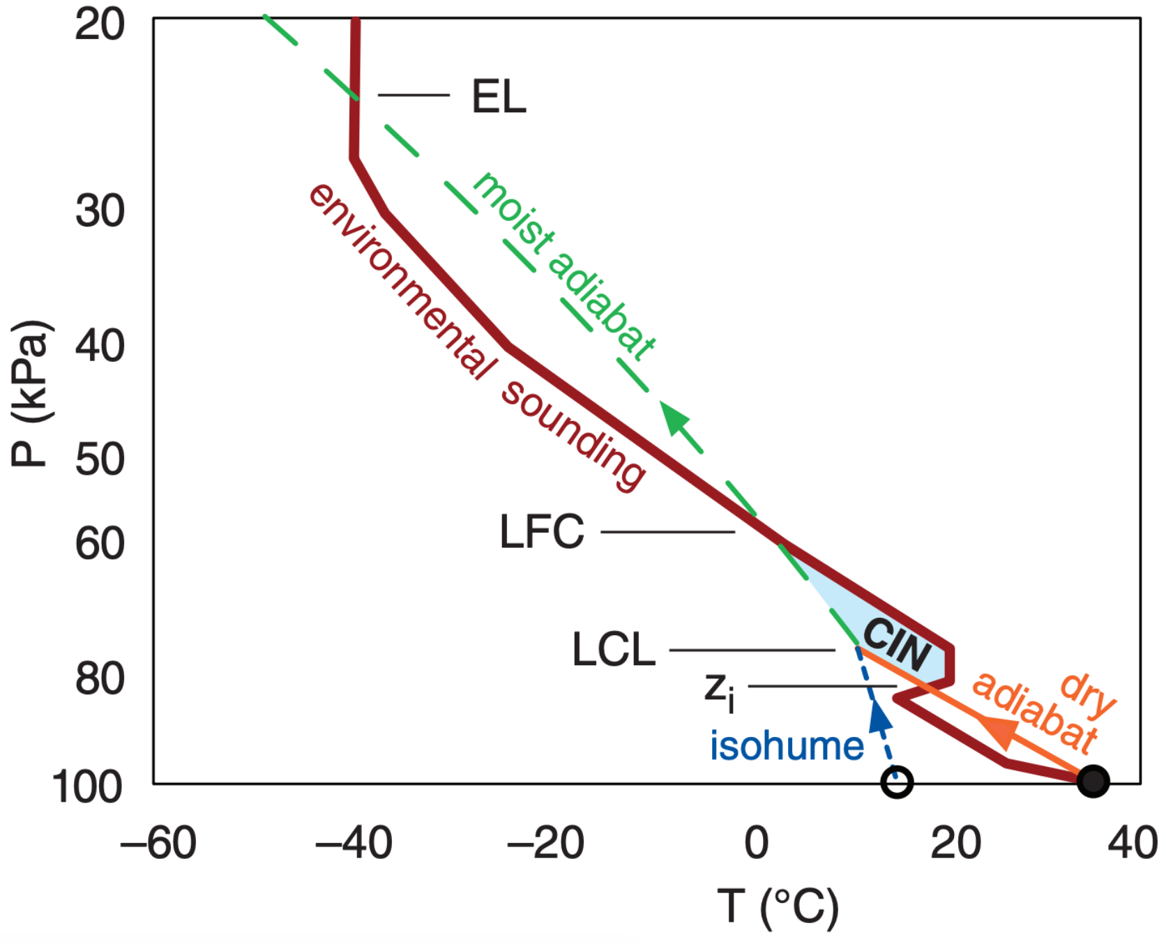
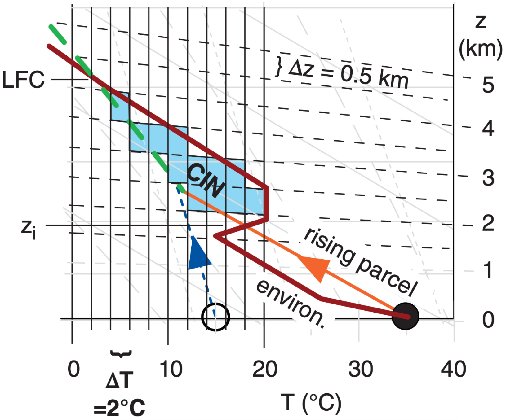
The total amount of work needed is proportional to the area shaded in Fig. 14.67. This work per unit mass is called the Convective Inhibition (CIN). The equation for CIN is identical to the equation for CAPE, except for the limits of the sum (i.e., z_i to LFC for CIN vs. LFC to EL for CAPE). Another difference is that CIN values are negative. CIN has units of J·kg^–1.

Figure 14.68 CIN based on max surface temperature and dew-point temperature forecasts and the early morning pre-storm sounding.

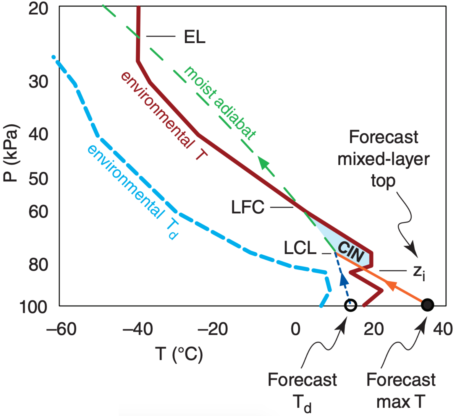
For the afternoon sounding of Fig. 14.67, CIN corresponds to the area between z_i and LFC, bounded by the dry and moist adiabats on the left and the environmental sounding on the right. For a morning sounding, a forecast of the afternoon’s high temperature provides the starting point for the rising air parcel, where z_i is the corresponding forecast for mixed-layer top (Fig. 14.68). Thus, for both Figs. 14.67 and 14.68, you can use:

\(\ \begin{align} C I N=\sum_{z_{i}}^{L F C} \frac{|g|}{T_{v e}}\left(T_{v p}-T_{v e}\right) \cdot \Delta z\tag{14.24}\end{align}\)

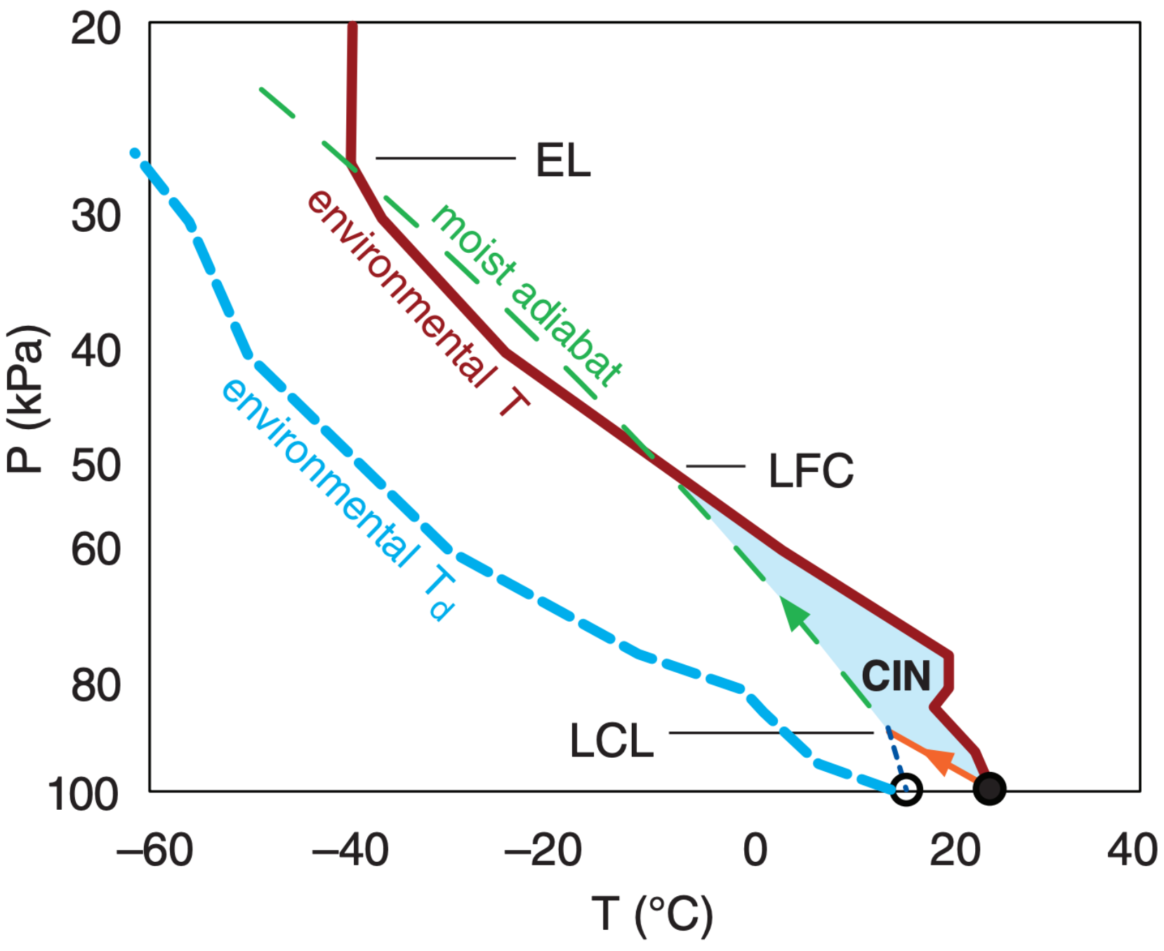
where T_v is virtual temperature, subscripts p and e indicate the air parcel and the environment, |g| = 9.8 m·s^–2 is the magnitude of gravitational acceleration, and ∆z is a height increment. Otherwise, CIN is usually found by summing between the surface (z = 0) and the LFC (Fig. 14.69).

\(\ \begin{align} C I N=\sum_{z=0}^{L F C} \frac{|g|}{T_{v e}}\left(T_{v p}-T_{v e}\right) \cdot \Delta z\tag{14.25}\end{align}\)

Figure 14.69 CIN between the surface and the LFC, for an early morning pre-storm sounding.

As before, if the virtual temperature is not known or is difficult to estimate, then often storm forecasters will use T in place of T_v in eq. (14.24) to get a rough estimate of CIN:

\(\ \begin{align} C I N=\sum_{z_{i}}^{L F C} \frac{|g|}{T_{e}}\left(T_{p}-T_{e}\right) \cdot \Delta z\tag{14.26}\end{align}\)

although this can cause errors as large as 35 J·kg–1 in the CIN value. Similar approximations can be made for eq. (14.25). Also, a mean-layer CIN (ML CIN) can be used, where the starting air parcel is based on average conditions in the bottom 1 km of air.

CIN is what prevents, delays, or inhibits formation of thunderstorms. Larger magnitudes of CIN (as in Fig. 14.69) are less likely to be overcome by trigger mechanisms, and are more effective at preventing thunderstorm formation. CIN magnitudes (Table 14-4) smaller than about 60 J·kg–1 are usually small enough to allow deep convection to form if triggered, but large enough to trap heat and humidity in the boundary layer prior to triggering, to serve as the thunderstorm fuel. CIN is the cap that must be broken to enable thunderstorm growth.

Storms that form in the presence of large CIN are less likely to spawn tornadoes. However, large CIN can sometimes be circumvented if an elevated trigger mechanism forces air-parcel ascent starting well above the surface.

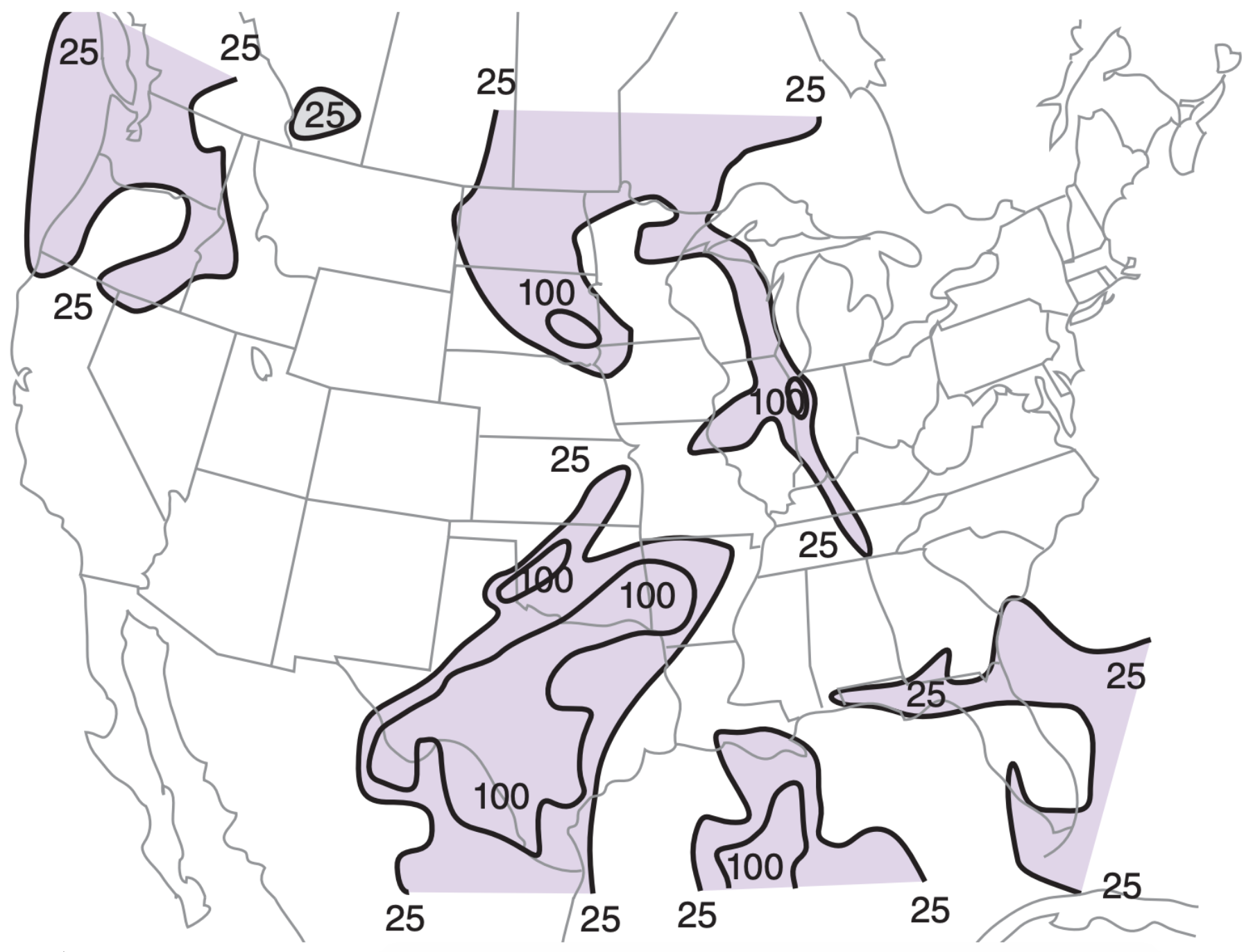
The area on a thermo diagram representing CIN is easily integrated by computer, and is often reported with the plotted sounding. [CAUTION: often the magnitude of CIN is reported (i.e., as a positive value).] CIN magnitudes from many sounding stations can be plotted on a weather map and analyzed, as in Fig. 14.70. To estimate CIN by hand, you can use the same tiling method as was done for CAPE (see the Sample Application at left).

Thunderstorms are more likely for smaller values of ∆z_cap, where ∆z_cap = z_LFC – z_LCL is the thickness of the nonlocally stable region at the bottom of the storm. A thinner cap on top of the ABL might allow thunderstorms to be more easily triggered.

Figure 14.70 Weather map similar to Fig. 14.38 over USA, but for magnitude of mean-layer convective inhibition energy (ML CIN) in J·kg^–1.

Table 14-4. Convective Inhibition (CIN)
CIN Value (J·kg^–1)	Interpretation
> 0	No cap. Allows weak convection.
0 to –20	Weak cap. Triggering easy. Air-mass thunderstorms possible.
–20 to –60	Moderate cap. Best conditions for CB. Enables fuel build-up in boundary layer. Allows most trigger mechanisms to initiate storm.
–60 to –100	Strong cap. Difficult to break. Need exceptionally strong trigger.
< –100	Intense cap. CB triggering unlikely.

Sample Application

Estimate the convective inhibition (CIN) value for the sounding of Fig. 14.25. Are thunderstorms likely?

Find the Answer

Given: Sounding of Fig. 14.25, as zoomed below.

Find: CIN = ? J·kg^–1.

Cover the CIN area with small tiles of size ∆z = 500 m and ∆T = –2°C (where the negative sign indicates the rising parcel is colder than the environmental sounding). Each tile has area = ∆T·∆z = –1,000 K·m. I count 12 tiles, so the total area is –12,000. Also, by eye the average environmental temperature in the CIN region is about T_e = 12°C = 285 K.

Use eq. (14.26): CIN = [(9.8 m s^–2)/(285 K)]·(–12,000 K·m) = –413 J·kg^–1.

From Table 14-4, thunderstorms are unlikely.

Check: By eye, the CIN area of Fig. 14.25 is about 1/5 the size of the CAPE area. Indeed, the answer above has about 1/5 the magnitude of CAPE (1976 J·kg^–1), as found in previous solved exercises. Units OK too.

Exposition: The negative CIN implies that work must be done ON the air to force it to rise through this region, as opposed to the positive CAPE values which imply that work is done BY the rising air.

14.6.2. Triggers

Any external process that forces boundary-layer air parcels to rise through the statically stable cap can be a trigger. Some triggers are:

• Boundaries between airmasses:
  • cold, warm, or occluded fronts,
  • gust fronts from other thunderstorms,
  • sea-breeze fronts,
  • dry lines.
• Other triggers:
  • the effects of mountains on winds,
  • small regions of high surface heating,
  • vertical oscillations called buoyancy waves.

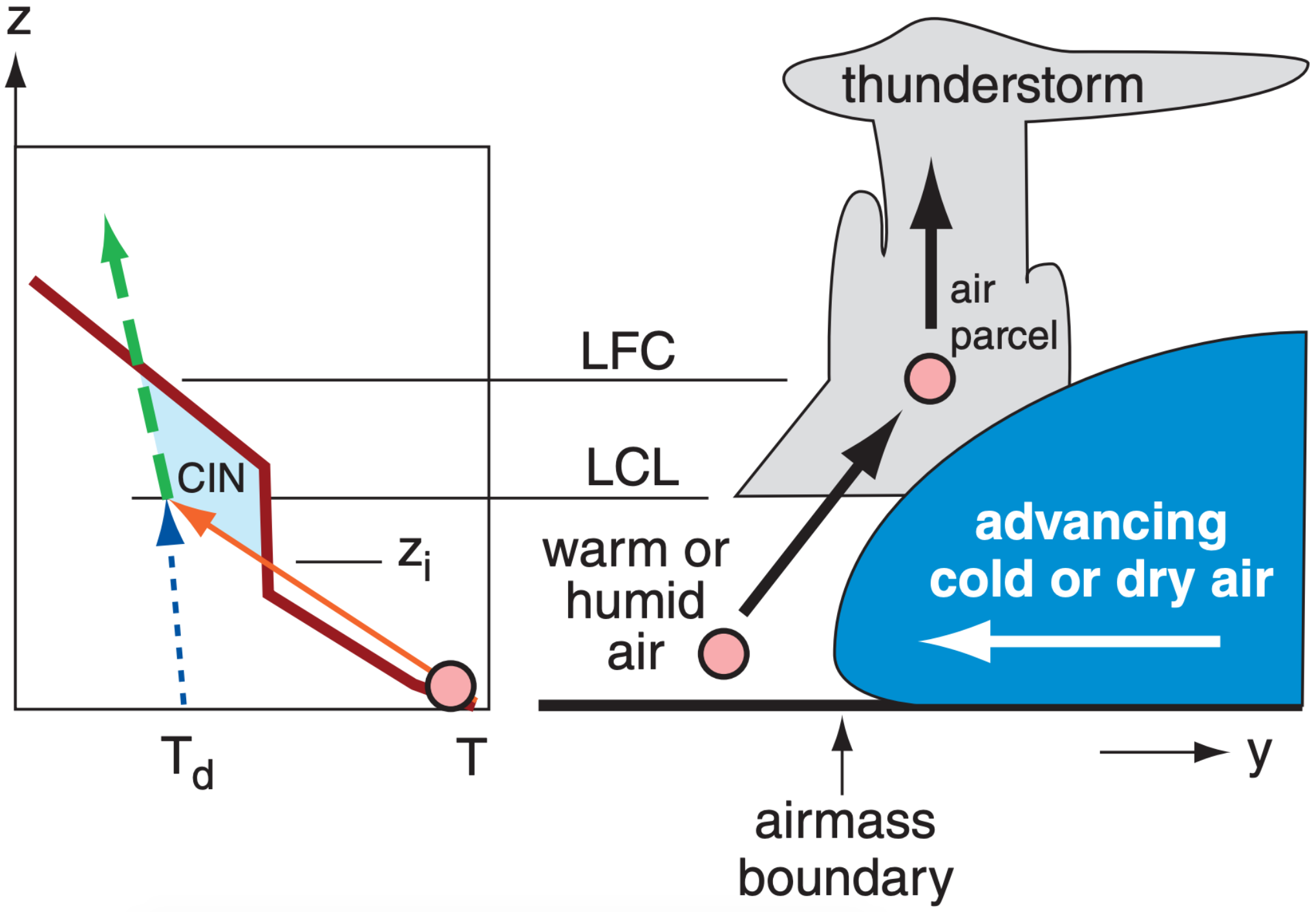
If one airmass is denser than an adjacent airmass, then any convergence of air toward the dividing line between the airmasses (called an airmass boundary) will force the less-dense air to rise over the denser air. A cold front is a good example (Fig. 14.71), where cold, dense air advances under the less-dense warm air, causing the warm air to rise past z_i .

Figure 14.71 Warmer or moister (less-dense) air forced to rise over advancing colder or drier (more-dense) air can trigger thunderstorms if the air parcels forced to rise reach their LFC. The portion of thunderstorm clouds between the LCL and the LFC can have a smooth or laminar appearance. Above the LFC the clouds look much more convective, with rising turrets that look like cauliflower.

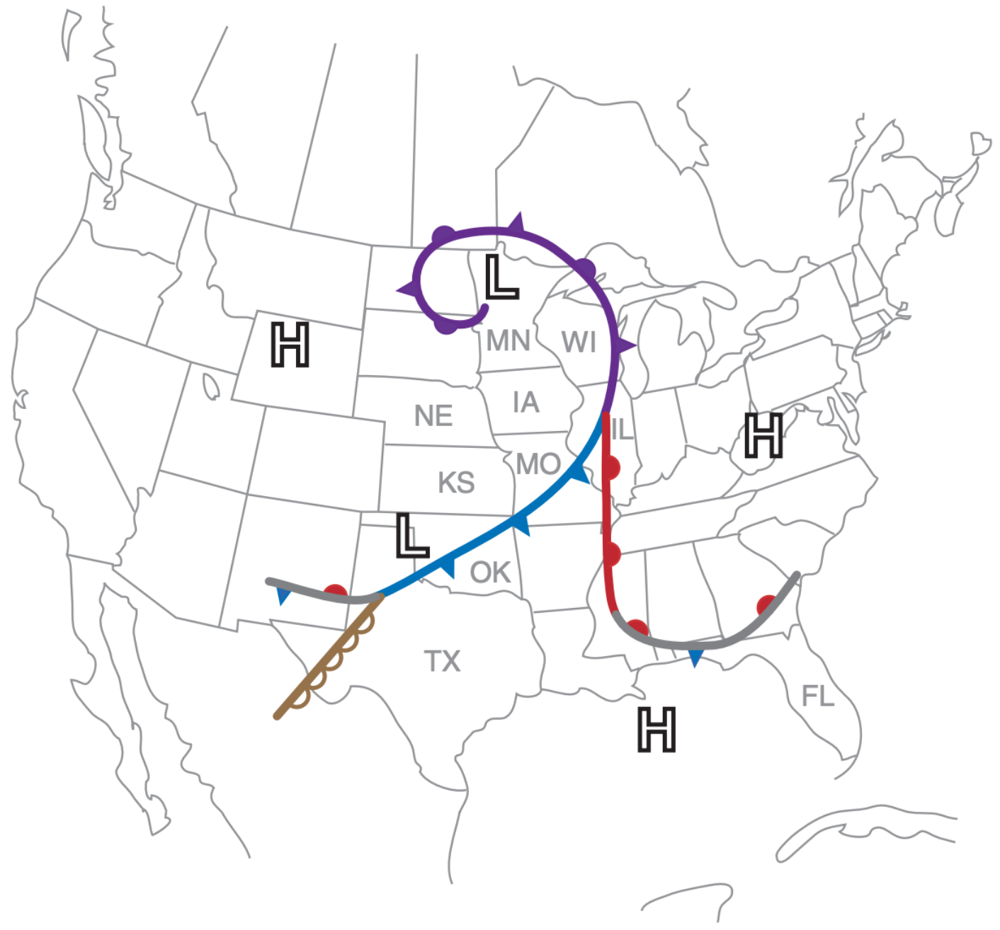
Surface-based cold and warm fronts are synoptically-forced examples of airmass boundaries. Upper-level synoptic fronts (with no signature on a surface weather map) can also cause lifting and trigger thunderstorms. Fig. 14.72 shows the frontal analysis for the 24 May 2006 case study that has been presented in many of the preceding sections. These frontal zones could trigger thunderstorms.

Figure 14.72 Synoptic frontal analysis over N. America at 22 UTC on 24 May 2006. An occluded front extends from a low (L) in Minnesota (MN) into Illinois (IL), where the warm and cold fronts meet. The cold front extends from IL through Oklahoma (OK) and Texas (TX), and merges with a dry line in SW Texas. (See Chapter 13 section 13.1 “Info” for identification of US states.)

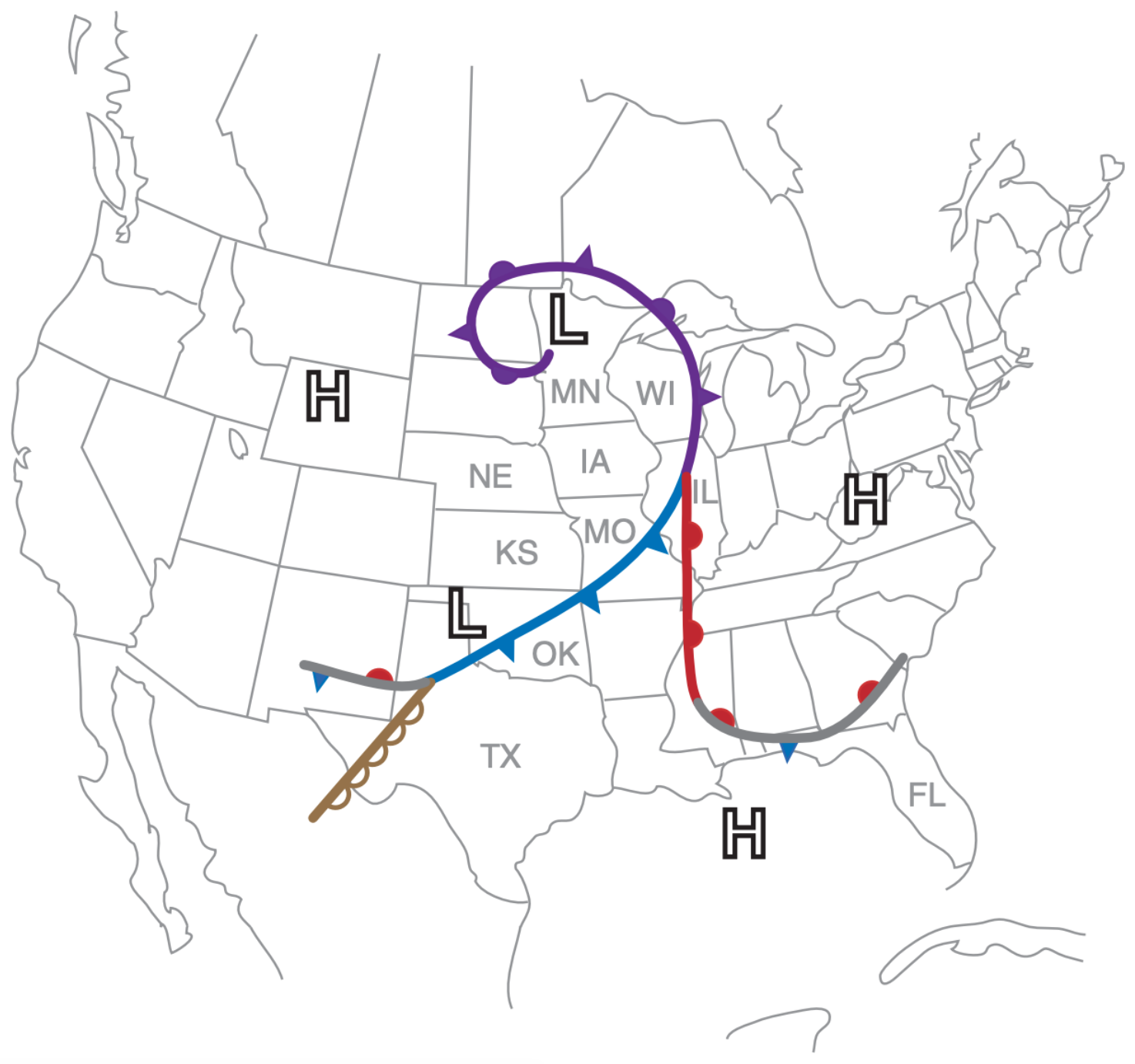
Sea-breeze (see the Regional Winds chapter) or lake-breeze fronts create a similar density discontinuity on the mesoscale at the boundary between the cool marine air and the warmer continental air during daytime, and can also trigger convection. If a cold downburst from a thunderstorm hits the ground and spreads out, the leading edge is a gust front of cooler, denser air that can trigger other thunderstorms (via the propagation mechanism already discussed). The dry line separating warm dry air from warm humid air is also an airmass boundary (Figs. 14.71 & 14.72), because dry air is more dense than humid air at the same temperature (see definition of virtual temperature in Chapter 1).

These airmass boundaries are so crucial for triggering thunderstorms that meteorologists devote much effort to identifying their presence. Lines of thunderstorms can form along them. Synoptic-scale fronts and dry lines are often evident from weather-map analyses and satellite images. Sea-breeze fronts and gust fronts can be seen by radar as convergence lines in the Doppler wind field, and as lines of weakly enhanced reflectivity due to high concentrations of insects (converging there with the wind) or a line of small cumulus clouds. When two or more air-mass boundaries meet or cross, the chance of triggering thunderstorms is greater such as over Illinois and Texas in the case-study example of Fig. 14.72.

Figure 14.72 Synoptic frontal analysis over N. America at 22 UTC on 24 May 2006. An occluded front extends from a low (L) in Minnesota (MN) into Illinois (IL), where the warm and cold fronts meet. The cold front extends from IL through Oklahoma (OK) and Texas (TX), and merges with a dry line in SW Texas. (See Chapter 13 section 13.1 “Info” for identification of US states.)

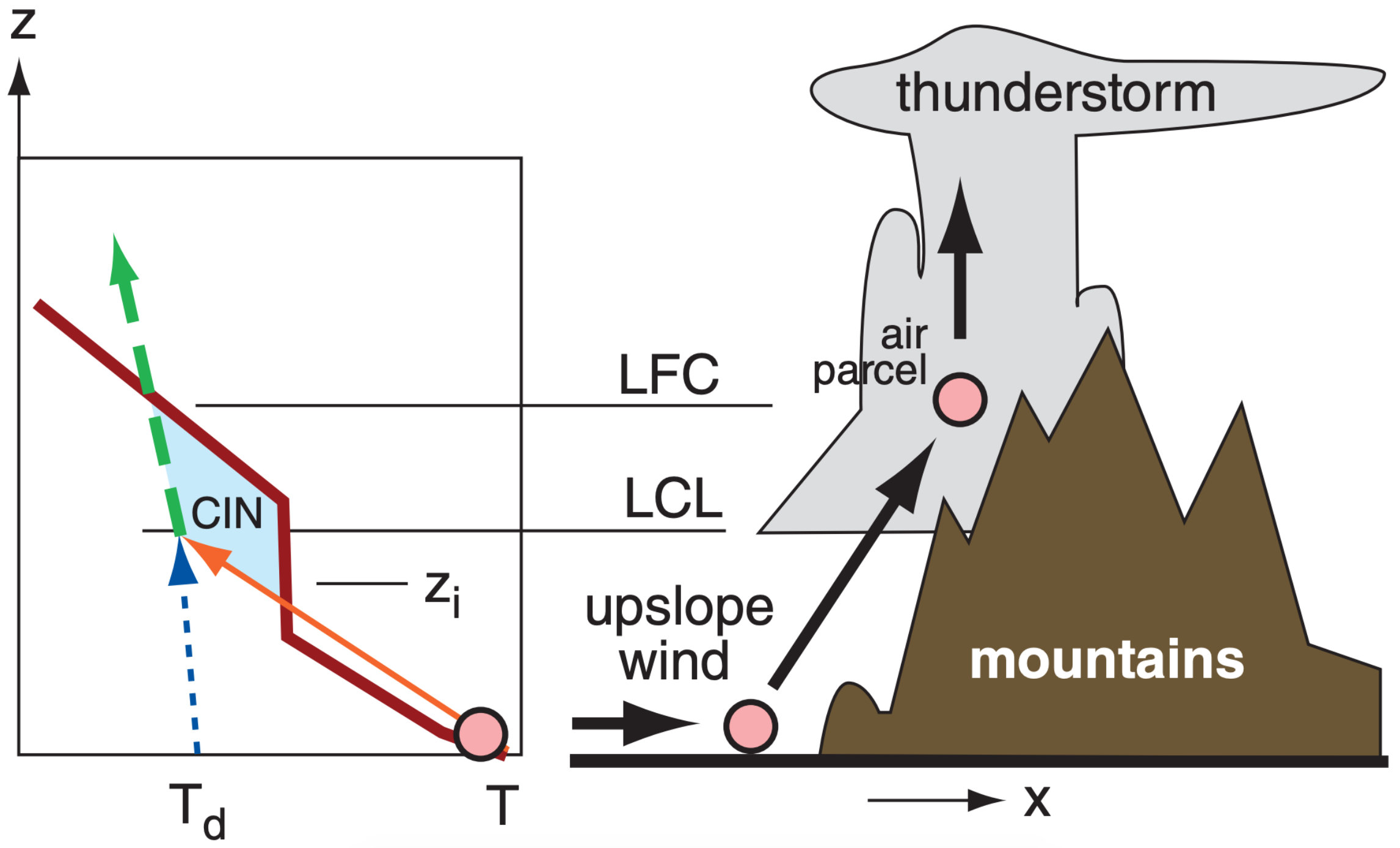
Horizontal winds hitting a mountain slope can be forced upward (Fig. 14.73), and can trigger orographic thunderstorms. Once triggered by the mountains, the storms can persist or propagate (by triggering daughter storms via their gust fronts) as they are blown away from the mountains by the steering-level winds.

Figure 14.73 Wind hitting a mountain can be forced upslope, triggering thunderstorms called orographic thunderstorms.

Figure 14.74 Thunderstorms generated in the updraft portions of buoyancy (gravity) waves.

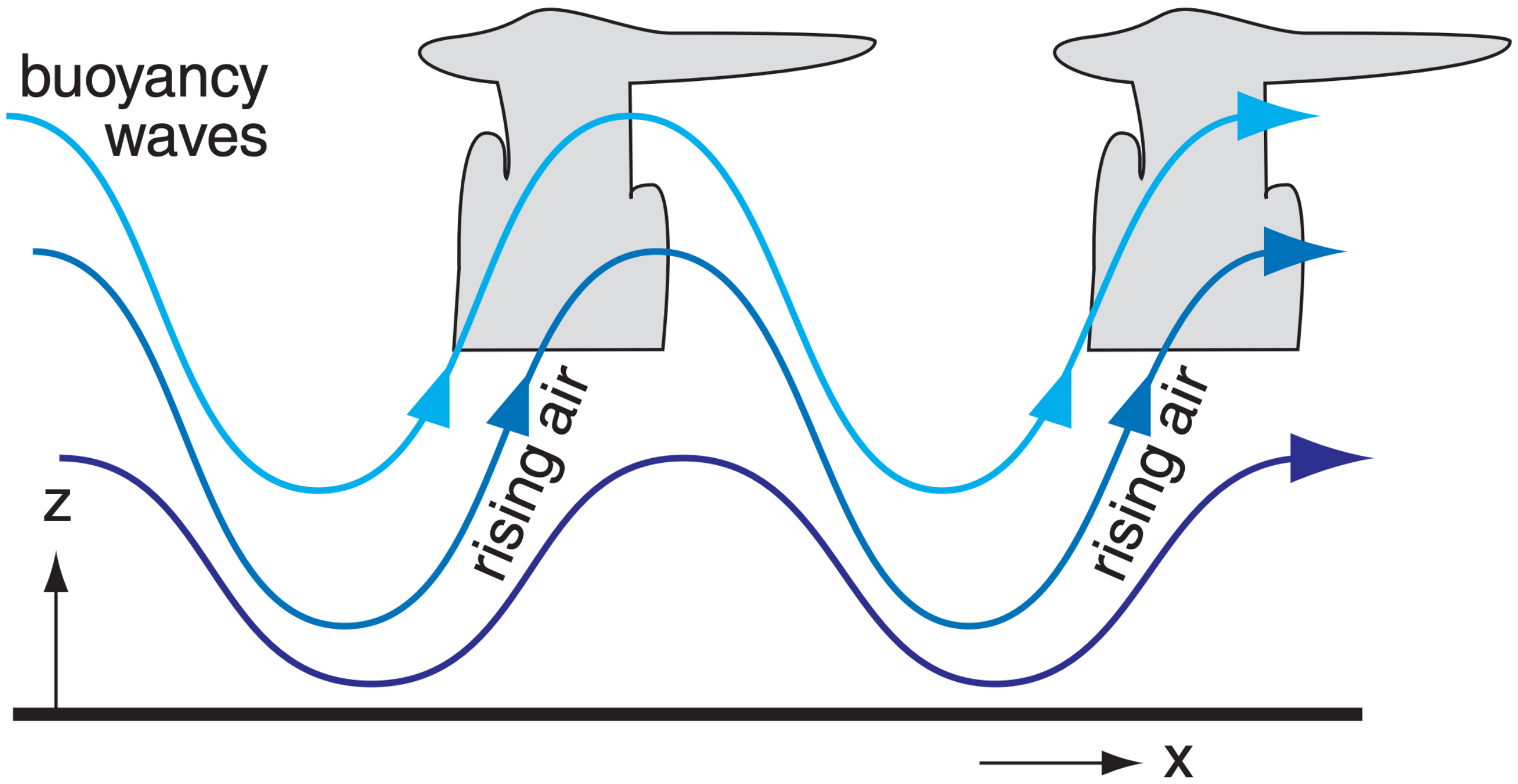
Sometimes when the air flows over mountains or is pushed out of the way by an advancing cold front, vertical oscillations called buoyancy waves or gravity waves (Fig. 14.74) can be generated in the air (see the Regional Winds chapter). If the lift in the updraft portion of a wave is sufficient to bring air parcels to their LFC, then thunderstorms can be triggered by these waves.

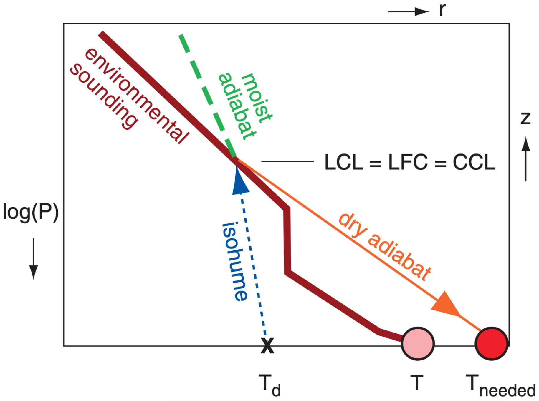
Another trigger is possible if the air near the ground is warmed sufficiently by its contact with the sun-heated Earth. The air may become warm enough to rise as a thermal through the cap and reach the LFC due to its own buoyancy. The temperature needed for this to happen is called the convective temperature, and is found as follows:

1. Plot the environmental sounding and the surface dew-point temperature (Fig. 14.75).
2. From T_d, follow the isohume up until it hits the sounding. This altitude is called the convective condensation level (CCL).
3. Follow the dry adiabat back to the surface to give the convective temperature needed.

You should forecast airmass thunderstorms to start when the surface air temperature is forecast to reach the convective temperature, assuming the environmental sounding above the boundary layer does not change much during the day. Namely, determine if the forecast high temperature for the day will exceed the convective temperature, and at what time this criterion will be met.

Often several triggering mechanisms work in tandem to create favored locations for thunderstorm development. For example, a jet streak may move across North America, producing upward motion under its left exit region and thereby reducing the strength of the cap as it passes (see the “Layer Method for Static Stability” section in the Atmospheric Stability chapter). If the jet streak crosses a region with large values of CAPE at the same time as the surface temperature reaches its maximum value, then the combination of these processes may lead to thunderstorm development.

Figure 14.75 The convective temperature needed so that an air parcel has no CIN, and can reach its LFC under its own buoyancy. CCL = convective condensation level.

Sample Application

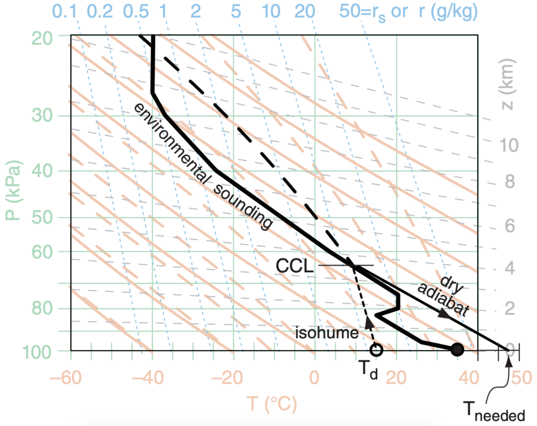
Use the sounding in Fig. 14.25 to find the convective temperature and the convective condensation level. Are thunderstorms likely to be triggered?

Find the Answer

Given: Fig. 14.25.

Find: P_CCL = ? kPa, T_needed = ? °C , yes/no Tstorms

Step 1: Plot the sounding (see next column).

Step 2: From the surface dew-point temperature, follow the isohume up until it hits the sounding to find the CCL. Thus: P_CCL ≈ 63 kPa ( or z_CCL ≈ 3.7 km).

Step 2: Follow the dry adiabat down to the surface, and read the temperature from the thermo diagram. T_needed ≈ 47 °C is the convective temperature.

Check: Values agree with figure.

Exposition: Typical high temperatures in the prairies of North America are unlikely to reach 47°C.

Thus, the triggering of a thunderstorm by a rising thermal is unlikely for this case. However, thunderstorms could be triggered by an airmass boundary such as a cold front, if the other conditions are met for thunderstorm formation.

Finally, a word of caution. As with each of the other requirements for a thunderstorm, triggering (lift) by itself is insufficient to create thunderstorms. Also needed are the instability, abundant moisture, and wind shear. To forecast thunderstorms you must forecast all four of the key ingredients. That is why thunderstorm forecasting is so difficult.