15.2: Gust Fronts and Downbursts

15.2.1. Attributes

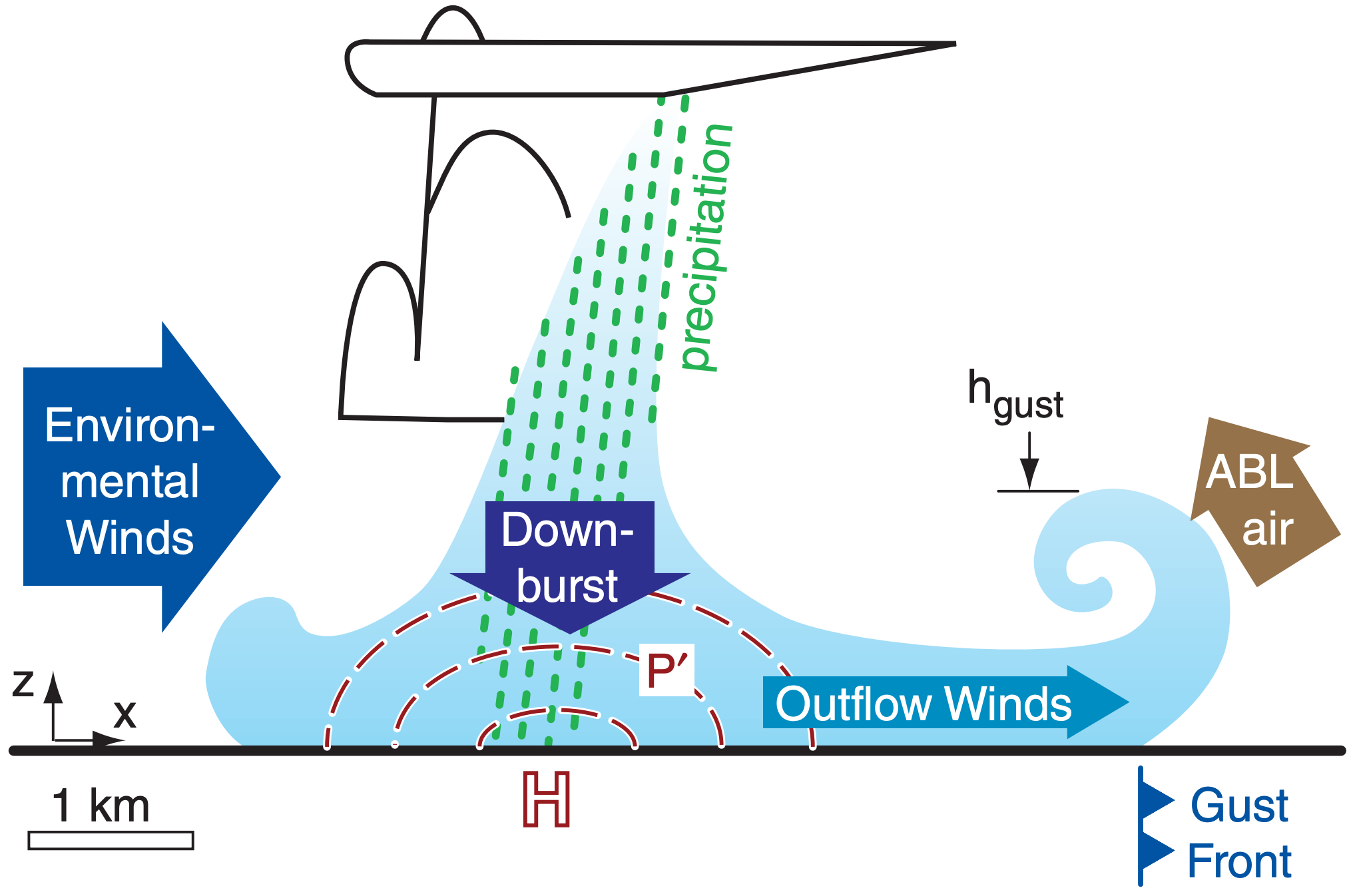
Downbursts are rapidly descending (w = –5 to –25 m s^–1) downdrafts of air (Fig. 15.11), found below clouds with precipitation or virga. Downbursts of 0.5 to 10 km diameter are usually associated with thunderstorms and heavy rain. Downburst speeds of order 10 m s^–1 have been measured 100 m AGL. The descending air can hit the ground and spread out as strong straight-line winds causing damage equivalent to a weak tornado (up to EF3 intensity). Smaller mid-level clouds (e.g., altocumulus with virga) can also produce downbursts that usually do not reach the ground.

Small diameter (1 to 4 km) downbursts that last only 2 to 5 min are called microbursts. Sometimes a downburst area will include one or more embedded microbursts.

Figure 15.11 Vertical slice through a thunderstorm downburst and its associated gust front. Light blue area indicates the rain-cooled air. Behind the gust front are non-tornadic (i.e., straight-line) outflow winds. H indicates location of meso-high pressure at the surface, and isobars of positive pressure perturbation P’ are dashed red lines. Dotted lines show precipitation. ABL is the warm, humid environmental air in the atmospheric boundary layer.

Acceleration of downburst velocity w is found by applying Newton’s 2nd law of motion to an air parcel:

\(\ \begin{align} \frac{\Delta w}{\Delta t} \approx-\frac{1}{\rho} \frac{\Delta P^{\prime}}{\Delta z}+|g| \cdot\left[\frac{\theta_{v}^{\prime}}{\theta_{v e}}-\frac{C_{v}}{C_{p}} \frac{P^{\prime}}{P_{e}}\right]\tag{15.5}\end{align}\)
\(\ Term: (A) \quad\quad\quad (B)\quad\quad\quad (C)\)

where w is negative for downdrafts, t is time, ρ is air density, P’ = P_parcel – P_e is pressure perturbation of the air parcel relative to the environmental pressure P_e, z is height, |g| = 9.8 m s^–2 is the magnitude of gravitational acceleration, θ_v’ = θ_{v parcel} – θ_ve is the deviation of the parcel’s virtual potential temperature from that of the environment θ_ve (in Kelvin), and C_v/C_p = 0.714 is the ratio of specific heat of air at constant volume to that at constant pressure.

Remember that the virtual potential temperature (from the Heat chapter) includes liquid-water and ice loading, which makes the air act as if it were colder, denser, and heavier. Namely, for the air parcel it is:

\(\ \begin{align} \theta_{v \text { parcel }}=\theta_{\text {parcel}} \cdot\left(1+0.61 \cdot r-r_{L}-r_{I}\right)_{\text {parcel}}\tag{15.6}\end{align}\)

where θ is air potential temperature (in Kelvin), r is water-vapor mixing ratio (in g g^–1, not g kg^–1), r_L is liquid water mixing ratio (in g g^–1), and rI is ice mixing ratio (in g g^–1). For the special case of an environment with no liquid water or ice, the environmental virtual potential temperature is:

\(\ \begin{align} \theta_{v e}=\theta_{e} \cdot(1+0.61 \cdot r)_{e}\tag{15.7}\end{align}\)

Equation (15.5) says that three forces (per unit mass) can create or enhance downdrafts. (A) Pressure-gradient force is caused when there is a difference between the pressure profile in the environment (which is usually hydrostatic) and that of the parcel. (B) Buoyant force combines the effects of temperature in the evaporatively cooled air, precipitation drag associated with falling rain drops or ice crystals, and the relatively lower density of water vapor. (C) Perturbation-pressure buoyancy force is where an air parcel of lower pressure than its surroundings experiences an upward force. Although this last effect is believed to be small, not much is really known about it, so we will neglect it here.

Evaporative cooling and precipitation drag are important for initially accelerating the air downward out of the cloud. We will discuss those factors first, because they can create downbursts. The vertical pressure gradient becomes important only near the ground. It is responsible for decelerating the downburst just before it hits the ground, which we will discuss in the “gust front” subsection.

15.2.2. Precipitation Drag on the Air

When hydrometeors (rain drops and ice crystals) fall at their terminal velocity through air, the drag between the hydrometeor and the air tends to pull some of the air with the falling precipitation. This precipitation drag produces a downward force on the air equal to the weight of the precipitation particles. For details on precipitation drag, see the Precipitation Processes Chapter.

This effect is also called liquid-water loading or ice loading, depending on the phase of the hydrometeor. The downward force due to precipitation loading makes the air parcel act heavier, having the same effect as denser, colder air. As was discussed in the Atmos. Basics and Heat Budgets chapters, use virtual temperature T_v or virtual potential temperature θ_v to quantify this effective cooling.

Sample Application

10 g kg^–1 of liquid water exists as rain drops in saturated air of temperature 10°C and pressure 80 kPa. The environmental air has a temperature of 10°C and mixing ratio of 4 g kg^–1. Find the: (a) buoyancy force per mass associated with air temperature and water vapor, (b) buoyancy force per mass associated with just the precipitation drag, and (c) the downdraft velocity after 1 minute of fall, due to only (a) and (b).

Find the Answer

Given: Parcel: r_L = 10 g kg^–1, T = 10°C, P = 80 kPa, Environ.: r = 4 g kg^–1, T = 10°C, P = 80 kPa, ∆t = 60 s. Neglect terms (A) and (C).

Find: (a) Term(Bdue to T & r) = ? N kg^–1,

(b) Term(Bdue to r_L & r_I ) = ? N kg^–1 (c) w = ? m s^–1

(a) Because the parcel air is saturated, r_parcel = r_s. Using a thermo diagram (because its faster than solving a bunch of equations), r_s ≈ 9.5 g kg^–1 at P = 80 kPa and T = 10°C. Also, from the thermo diagram, θ_parcel ≈ 28°C = 301 K. Thus, using the first part of eq. (15.6):

θ_{v parcel} ≈ (301 K)·[1 + 0.61·(0.0095 g g^–1)] ≈ 302.7 K

For the environment, also θ ≈ 28°C = 301 K, but r = 4 g kg^–1. Thus, using eq. (15.7):

θ_ve ≈ (301 K)·[1 + 0.61·(0.004 g g^–1)] ≈ 301.7 K

Use eq. (15.5): Term(B_{due to T & r}) = |g|·[ ( θ_{v parcel} – θ_ve ) / θ_ve ] = (9.8 m s^–2)·[ (302.7 – 301.7 K) / 301.7 K ] = 0.032 m s^–2 = 0.032 N kg^–1.

(b) Because r_I was not given, assume r_I = 0 everywhere, and r_L = 0 in the environment.

Term(B_{due to rL & rI} ) = –|g|·[ (r_L + r_I )_parcel – (r_L + r_I )_e]. = – (9.8 m s^–2)·[ 0.01 g g^–1 ] = –0.098 N kg^–1.

(c) Assume initial vertical velocity is zero.

Use eq. (15.5) with only Term B: ( w_final – w_initial )/ ∆t = [Term(B_T & _r) + Term(B_rL & r_I )]

w_final = (60 s)·[ 0.032 – 0.098 m s^–2 ] ≈ –4 m s^–1.

Check: Units OK. Physics OK.

Exposition: Although the water vapor in the air adds buoyancy equivalent to a temperature increase of 1°C, the liquid-water loading decreases buoyancy, equivalent to a temperature decrease of 3°C. The net effect is that this saturated, liquid-water laden air acts 2°C colder and heavier than dry air at the same T.

CAUTION. The final vertical velocity assumes that the air parcel experiences constant buoyancy forces during its 1 minute of fall. This is NOT a realistic assumption, but it did make the exercise a bit easier to solve. In fact, if the rain-laden air descends below cloud base, then it is likely that the rain drops are in an unsaturated air parcel, not saturated air as was stated for this exercise. We also neglected turbulent drag of the downburst air against the environmental air. This effect can greatly reduce the actual downburst speed compared to the idealized calculations above.

15.2.3. Cooling due to Droplet Evaporation

Three factors can cause the rain-filled air to be unsaturated. (1) The rain can fall out of the thunderstorm into drier air (namely, the rain moves through the air parcels, not with the air parcels). (2) As air parcels descend in the downdraft (being dragged downward by the rain), the air parcels warm adiabatically and can hold more vapor. (3) Mixing of the rainy air with the surrounding drier environment can result in a mixture with lowered humidity.

Raindrops can partially or totally evaporate in this unsaturated air, converting sensible heat into latent heat. Namely, air cools as the water evaporates, and cool air has negative buoyancy. Negatively buoyant air sinks, creating downbursts of air. One way to quantify the cooling is via the change of potential temperature associated with evaporation of ∆rL (g_liq.water kg_air^–1) of liquid water:

\(\ \begin{align} \Delta \theta_{\text {parcel}}=\left(L_{v} / C_{p}\right) \cdot \Delta r_{L}\tag{15.8}\end{align}\)

where (L_v/C_p) = 2.5 K·kg^air·(g_water)^–1, and where ∆r_L = r_{L final} – r_{L initial} is negative for evaporation. This parcel cooling enters the downdraft-velocity equation via θ_parcel in eq. (15.6).

Figure 15.12 Rain drops reduce the virtual potential temperature of the air by both their weight (precipitation drag) and cooling as they evaporate. ∆θ_v is the change of virtual potential temperature compared to air containing no rain drops initially. r_L is liquid-water mixing ratio for the drops in air. For any initial r_L along the vertical axis, the blue dot indicates the ∆θ_v due to only liquid water loading. As that same raindrop evaporates, follow the diagonal line down to see changes in both r_L and ∆θ_v.

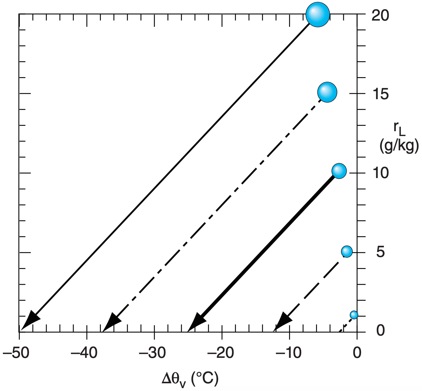
Precipitation drag is usually a smaller effect than evaporative cooling. Fig. 15.12 shows both the precipitation-drag effect for different initial liquidwater mixing ratios (the black dots), and the corresponding cooling and liquid-water decrease as the drops evaporate. For example, consider the black dot corresponding to an initial liquid water loading of 10 g kg^–1. Even before that drop evaporates, the weight of the rain decreases the virtual potential temperature by about 2.9°C. However, as that drop evaporates, it causes a much larger amount of cooling to due latent heat absorption, causing the virtual-potential-temperature to decrease by 25°C after it has completely evaporated.

Evaporative cooling can be large in places where the environmental air is dry, such as in the high-altitude plains and prairies of the USA and Canada. There, raining convective clouds can create strong downbursts, even if all the precipitation evaporates before reaching the ground (i.e., for virga).

Downbursts are hazardous to aircraft in two ways. (1) The downburst speed can be faster than the climb rate of the aircraft, pushing the aircraft towards the ground. (2) When the downburst hits the ground and spreads out, it can create hazardous changes between headwinds and tailwinds for landing and departing aircraft (see the “Aircraft vs. Downbursts” INFO Box in this section.) Modern airports are equipped with Doppler radar and/or wind-sensor arrays on the airport grounds, so that warnings can be given to pilots.

Sample Application

For data from the previous Sample Application, find the virtual potential temperature of the air if:

a) all liquid water evaporates, and

b) no liquid water evaporates, leaving only the precipitation-loading effect.

c) Discuss the difference between (a) and (b)

Find the Answer

Given: r_L = 10 g kg^–1 initially. r_L = 0 finally.

Find: (a) ∆θ_parcel = ? K (b) ∆θ_{v parcel} = ? K

(a) Use eq. (15.8): ∆θ_parcel = [2.5 K·kg_air·(g_water)^–1] · (–10 g kg^–1) = –25 K

(b) From the Exposition section of the previous Sample Application:

∆θ_{v parcel precip. drag} = –3 K initially

Thus, the change of virtual potential temperature (between before and after the drop evaporates) is

∆θ_{v parcel} = ∆θ_{v parcel final} – ∆θ_{v parcel initial}

= – 25K – (–3 K) = –22 K.

Check: Units OK. Physics OK.

Exposition: (c) The rain is more valuable to the downburst if it all evaporates.

15.2.4. Downdraft CAPE (DCAPE)

Eq. (15.5) applies at any one altitude. As precipitation-laden air parcels descend, many things change. The descending air parcel cools and loses some of its liquid-water loading due to evaporation, thereby changing its virtual potential temperature. It descends into surroundings having different virtual potential temperature than the environment where it started. As a result of these changes to both the air parcel and its environment, the θ_v’ term in eq. (15.5) changes.

To account for all these changes, find term B from eq. (15.5) at each depth, and then sum over all depths to get the accumulated effect of evaporative cooling and precipitation drag. This is a difficult calculation, with many uncertainties.

An alternative estimate of downburst strength is via the Downdraft Convective Available Potential Energy (DCAPE, see shaded area in Fig. 15.13):

\(\ \begin{align} D C A P E=\sum_{z=0}^{z_{I F S}}|g| \frac{\theta_{v p}-\theta_{v e}}{\theta_{v e}} \cdot \Delta z\tag{15.9}\end{align}\)

where |g| = 9.8 m s^–2 is the magnitude of gravitational acceleration, θ_vp is the parcel virtual potential temperature (including temperature, water vapor, and precipitation-drag effects), θ_ve is the environment virtual potential temperature (Kelvin in the denominator), ∆z is a height increment to be used when conceptually covering the DCAPE area with tiles of equal size.

Figure 15.13 Thermo diagram (Theta-z diagram from the Stability chapter) example of Downdraft Convective Available Potential energy (DCAPE, yellow shaded area). Thick solid red line is environmental sounding. Black dot shows virtual potential temperature after top of environmental sounding has been modified by liquid-water loading caused by precipitation falling into it from above. Three scenarios of rain-filled air-parcel descent are shown: (a) no evaporative cooling, but only constant liquid water loading (thin solid line following a dry adiabat); (b) an initially saturated air parcel with evaporative cooling of the rain (dashed green line following a moist adiabat); and (c) partial evaporation (thick dotted black line) with a slope between the moist and dry adiabats.

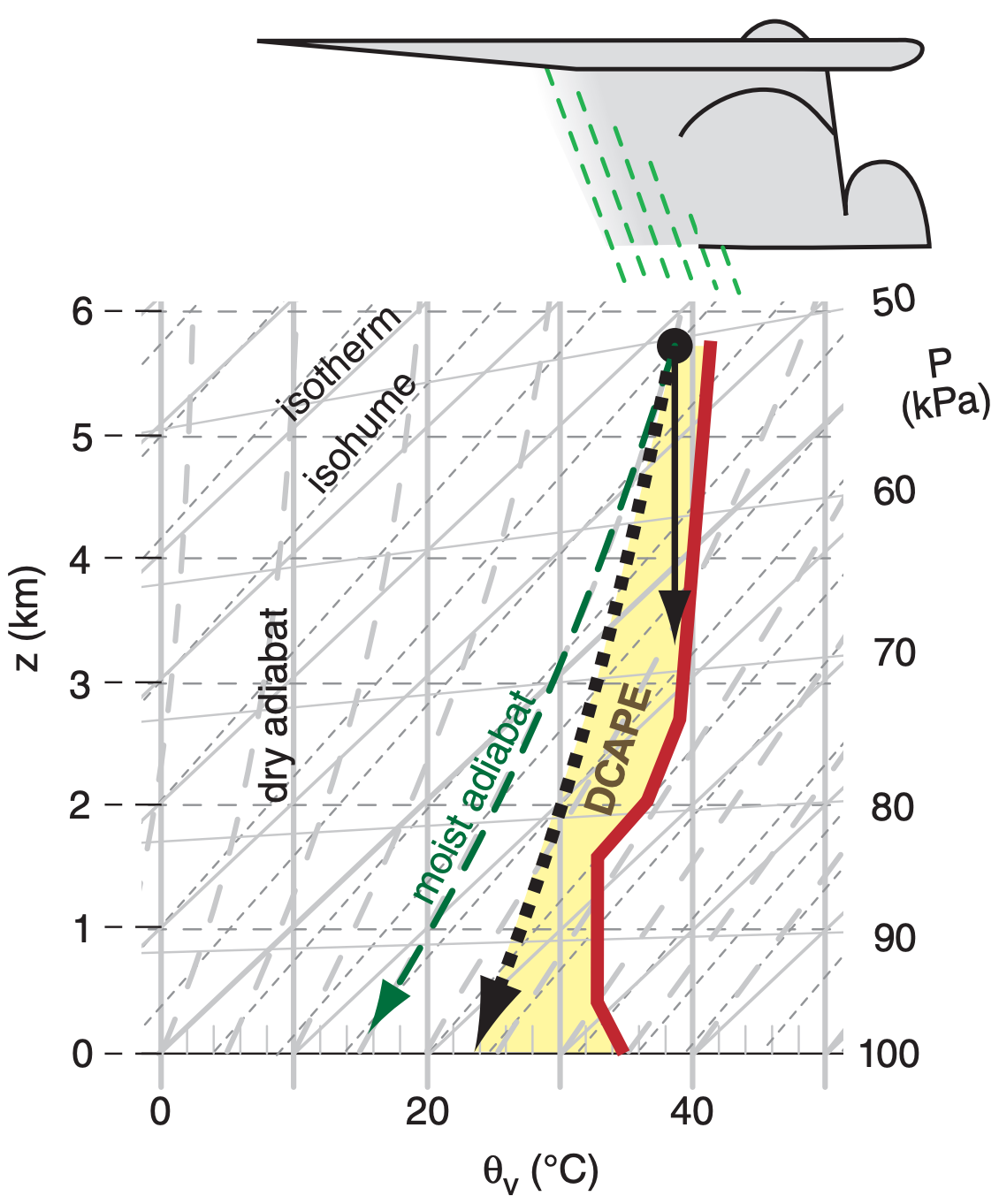
The altitude z_LFS where the precipitation-laden air first becomes negatively buoyant compared to the environment is called the level of free sink (LFS), and is the downdraft equivalent of the level of free convection. If the downburst stays negatively buoyant to the ground, then the bottom limit of the sum is at z = 0, otherwise the downburst would stop at a downdraft equilibrium level (DEL) and not be felt at the ground. DCAPE is negative, and has units of J kg^–1 or m² s^–2.

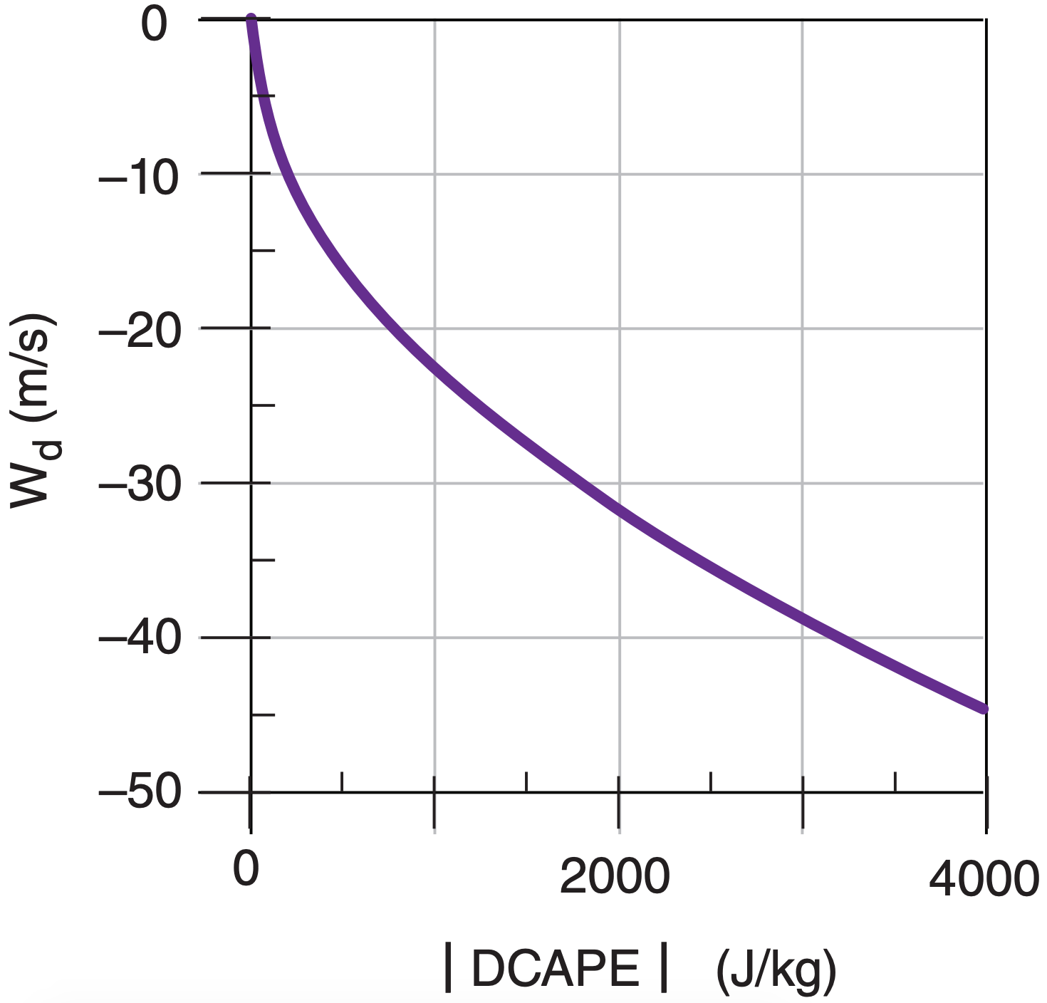
By relating potential energy to kinetic energy, the downdraft velocity is approximately:

\(\ \begin{align} w_{\max d o w n}=-(2 \cdot|D C A P E|)^{1 / 2}\tag{15.10}\end{align}\)

Air drag of the descending air parcel against its surrounding environmental air could reduce the likely downburst velocity w_d to about half this max value (Fig. 15.14):

\(\ \begin{align} w_{d}=w_{\max\ d o w n} / 2\tag{15.11}\end{align}\)

Figure 15.14 Downburst velocity w_d driven by DCAPE

Stronger downdrafts and associated straight-line winds near the ground are associated with larger magnitudes of DCAPE. For example, Fig. 15.15 shows a case study of DCAPE magnitudes valid at 22 UTC on 24 May 2006.

Figure 15.15 Example of downdraft DCAPE magnitude (J kg^–1) for 22 UTC 24 May 06 over the USA.

Sample Application

For the shaded area in Fig. 15.13, use the tiling method to estimate the value of DCAPE. Also find the maximum downburst speed and the likely speed.

Find the Answer

Given: Fig. 15.13, reproduced here.

Find: DCAPE = ? m² s^–2, wmax down = ? m s^–1 w_d = ? m s^–1

The DCAPE equation (15.9) can be re-written as

DCAPE = –[|g|/θ_ve]·(shaded area)

Method: Overlay the shaded region with tiles:

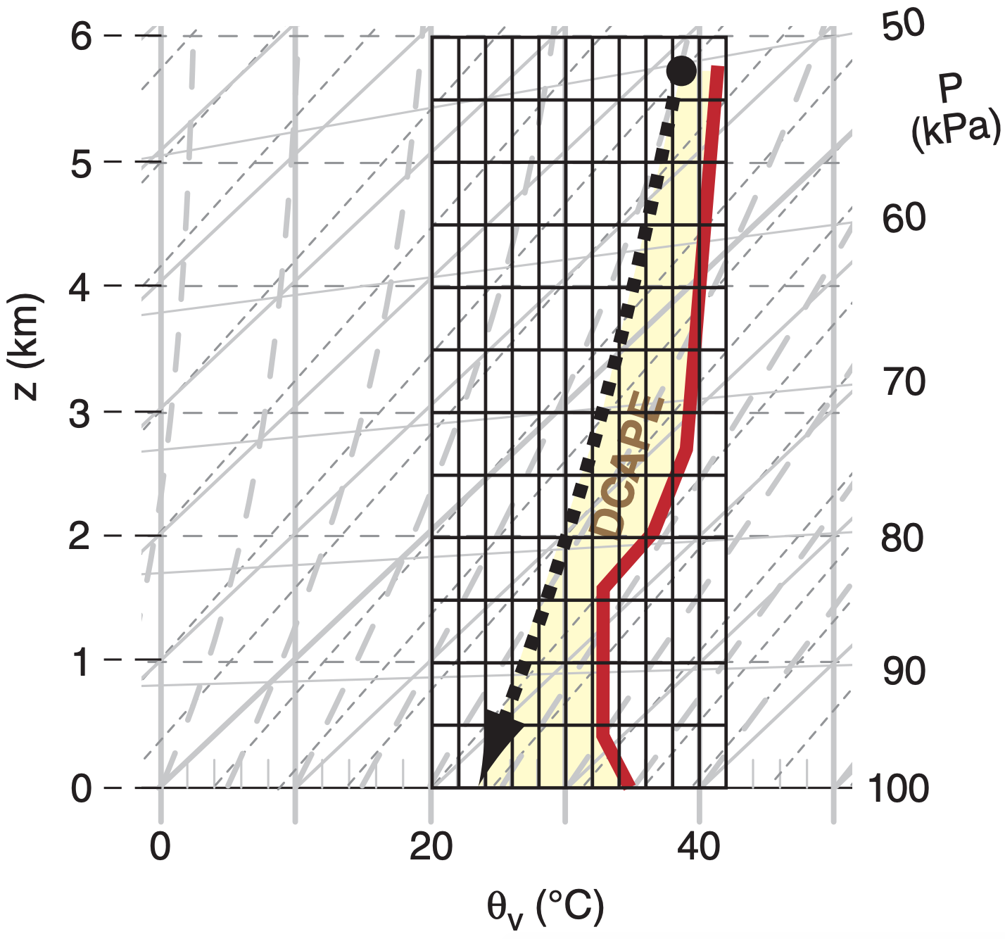
Each tile is 2°C = 2 K wide by 0.5 km tall (but you could pick other tile sizes instead). Hence, each tile is worth 1000 K·m. I count approximately 32 tiles needed to cover the shaded region. Thus:

(shaded area) = 32 x 1000 K·m = 32,000 K·m.

Looking at the plotted environmental sounding by eye, I estimate the average θ_ve = 37°C = 310 K.

DCAPE = –[(9.8 m s^–2)/310K]·(32,000 K·m) = –1012 m² s^–2

Next, use eq. (15.10):

w_{max down} = –[ 2 ·|–1012 m² s^–2 |]^1/2 = –45 m s^–1

Finally, use eq. (15.11):

w_d = w_{max down}/2 = –22.5 m s^–1.

Check: Units OK. Physics OK. Drawing OK.

Exposition: While this downburst speed might be observed 1 km above ground, the speed would diminish closer to the ground due to an opposing pressure-perturbation gradient. Since the DCAPE method doesn’t account for the vertical pressure gradient, it shouldn’t be used below about 1 km altitude.

INFO • CAPE vs. DCAPE

Although DCAPE shares the same conceptual framework as CAPE, there is virtually no chance of practically utilizing DCAPE, whereas CAPE is very useful. Compare the two concepts.

For CAPE: The initial state of the rising air parcel is known or fairly easy to estimate from surface observations and forecasts. The changing thermodynamic state of the parcel is easy to anticipate; namely, the parcel rises dry adiabatically to its LCL, and rises moist adiabatically above the LCL with vapor always close to its saturation value. Any excess water vapor instantly condenses to keep the air parcel near saturation. The resulting liquid cloud droplets are initially carried with the parcel.

For DCAPE: Both the initial air temperature of the descending air parcel near thunderstorm base and the liquid-water mixing ratio of raindrops are unknown. The raindrops don’t move with the air parcel, but pass through the air parcel from above. The air parcel below cloud base is often NOT saturated even though there are raindrops within it. The temperature of the falling raindrops is often different than the temperature of the air parcel it falls through. There is no requirement that the adiabatic warming of the air due to descent into higher pressure be partially matched by evaporation from the rain drops (namely, the thermodynamic state of the descending air parcel can be neither dry adiabatic nor moist adiabatic).

Unfortunately, the exact thermodynamic path traveled by the descending rain-filled air parcel is unknown, as discussed in the INFO box. Fig. 15.13 illustrates some of the uncertainty in DCAPE. If the rain-filled air parcel starting at pressure altitude of 50 kPa experiences no evaporation, but maintains constant precipitation drag along with dry adiabatic warming, then the parcel state follows the thin solid arrow until it reaches its DEL at about 70 kPa. This would not reach the ground as a down burst.

If a descending saturated air parcel experiences just enough evaporation to balance adiabatic warming, then the temperature follows a moist adiabat, as shown with the thin dashed line. But it could be just as likely that the air parcel follows a thermodynamic path in between dry and moist adiabat, such as the arbitrary dotted line in that figure, which hits the ground as a cool but unsaturated downburst.

15.2.5. Pressure Perturbation

As the downburst approaches the ground, its vertical velocity must decelerate to zero because it cannot blow through the ground. This causes the dynamic pressure to increase (P’ becomes positive) as the air stagnates.

Rewriting Bernoulli’s equation (see the Regional Winds chapter) using the notation from eq. (15.5), the maximum stagnation pressure perturbation P’ max at the ground directly below the center of the downburst is:

\(\ \begin{align} P_{\max }^{\prime}=\rho \cdot\left[\frac{w_{d}^{2}}{2}-\frac{|g| \cdot \theta_{v}^{\prime} \cdot z}{\theta_{v e}}\right]\tag{15.12}\end{align}\)
\(\ Term:\quad \quad(A)\quad\quad(B)\)

where ρ is air density, w_d is likely peak downburst speed at height z well above the ground (before it feels the influence of the ground), |g| = 9.8 m s^–2 is gravitational acceleration magnitude, and virtual potential temperature depression of the air parcel relative to the environment is θ_v’ = θ_{v parcel} – θ_ve .

Term (A) is an inertial effect. Term (B) includes the role of the added weight of cold air (with possible precipitation loading) in increasing the pressure [because θ_v’ is usually (but not always) negative in downbursts]. Both effects create a mesoscale high (mesohigh, H) pressure region centered on the downburst. Fig. 15.16 shows the solution to eq. (15.12) for a variety of different downburst velocities and virtual potential temperature deficits. Typical magnitudes are on the order of 0.1 to 0.6 kPa (or 1 to 6 mb) higher than the surrounding pressure.

Figure 15.16 Descending air of velocity wd decelerates to zero when it hits the ground, causing a pressure increase P’_max at the ground under the downburst compared to the surrounding ambient atmosphere. For descending air of the same temperature as its surroundings, the result from Bernoulli’s equation is plotted as the thick solid black line. If the descending air is also cold (i.e., has some a virtual potential temperature deficit –θ_v’ at starting altitude z), then the blue curves show how the pressure perturbation increases further.

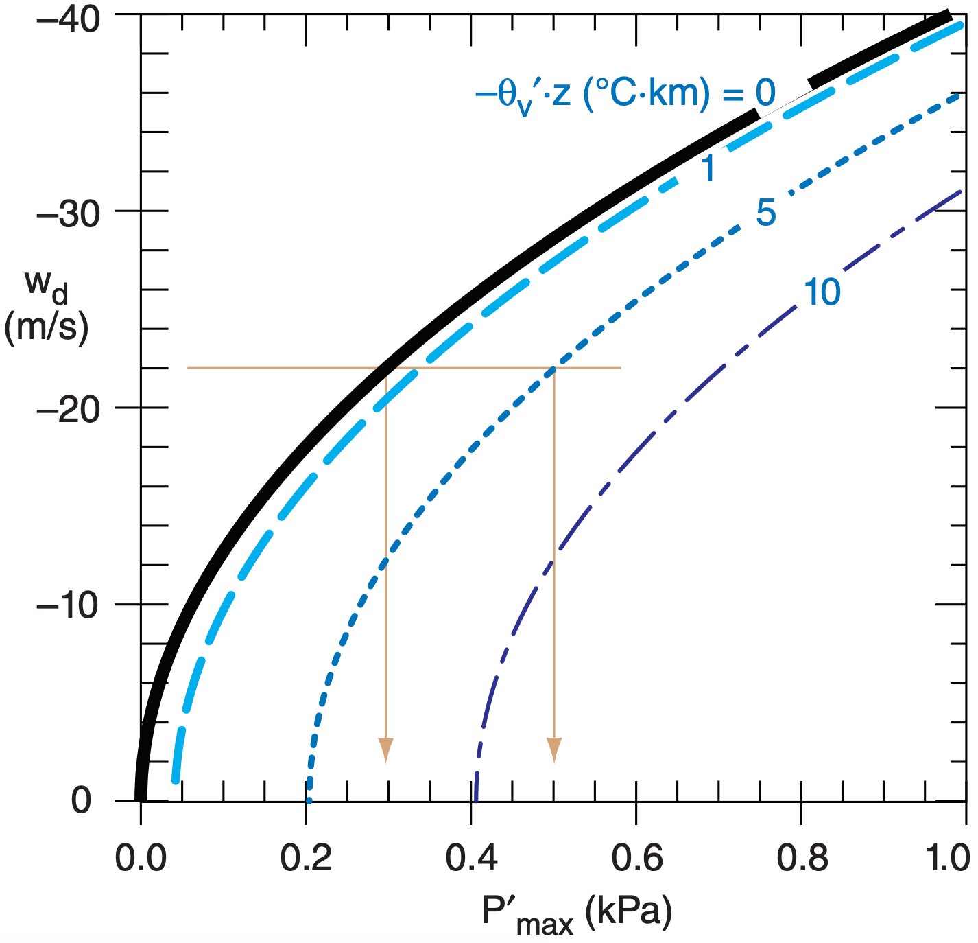
As you move away vertically from the ground and horizontally from the downburst center, the pressure perturbation decreases, as suggested by the dashed line isobars in Figs. 15.11 and 15.17. The vertical gradient of this pressure perturbation decelerates the downburst near the ground. The horizontal gradient of the pressure perturbation accelerates the air horizontally away from the downburst, thus preserving air-mass continuity by balancing vertical inflow with horizontal outflow of air.

Sample Application

A downburst has velocity –22 m s^–1 at 1 km altitude, before feeling the influence of the ground. Find the corresponding perturbation pressure at ground level for a downburst virtual potential temperature perturbation of (a) 0, and (b) –5°C.

Find the Answer

Given: w_d = –22 m s^–1, z = 1 km, θ_v’ = (a) 0, or (b) –5°C

Find: P’ _max = ? kPa

Assume standard atmosphere air density at sea level

ρ = 1.225 kg m^–3

Assume θ_ve = 294 K. Thus |g|/θ_ve = 0.0333 m·s^-2·K^-1

Use eq. (15.12):

(a) P’ _max = (1.225 kg m^–3)·[ (–22 m s^–1)²/₂ – 0 ] = 296 kg·m^–1·s^–2 = 296 Pa = 0.296 kPa

(b) θ_v’ = –5°C = –5 K because it represents a temperature difference.

P’ _max = (1.225 kg m^–3)· [ (–22 m s^–1)²/₂ – (0.0333 m·s^-2·K^-1)·(–5 K)·(1000 m)]

P’ _max = [ 296 + 204 ] kg·m^–1·s^–2 = 500 Pa = 0.5 kPa

Check: Units OK. Physics OK. Agrees with Fig. 15.16.

Exposition: For this case, the cold temperature of the downburst causes P’ to nearly double compared to pure inertial effects. Although P’ _max is small, P’ decreases to 0 over a short distance, causing large ∆P’/∆x & ∆P’/∆z. These large pressure gradients cause large accelerations of the air, including the rapid deceleration of the descending downburst air, and the rapid horizontal acceleration of the same air to create the outflow winds.

15.2.6. Outflow Winds & Gust Fronts

Driven by the pressure gradient from the meso-high,the near-surface outflow air tends to spread out in all directions radially from the downburst. It can be enhanced or reduced in some directions by background winds (Fig. 15.17). Straight-line outflow winds (i.e., non-tornadic; non-rotating) behind the gust front can be as fast as 35 m s^–1, and can blow down trees and destroy mobile homes. Such winds can make a howling sound called aeolian tones, as wake eddies form behind wires and twigs.

Figure 15.17 Horizontal slice through the air just above the ground, corresponding to Fig. 15.11. Shown are the downburst of average radius r (dark blue), gust front of average radius R (blue arc, with cold-frontal symbols [triangles]), cool air (gradient shaded light blue), and outflow winds (thick blue arrows) flowing in straight lines. H shows the location of a meso-high-pressure center near the ground, and the dashed red lines show isobars of positive perturbation pressure P’.

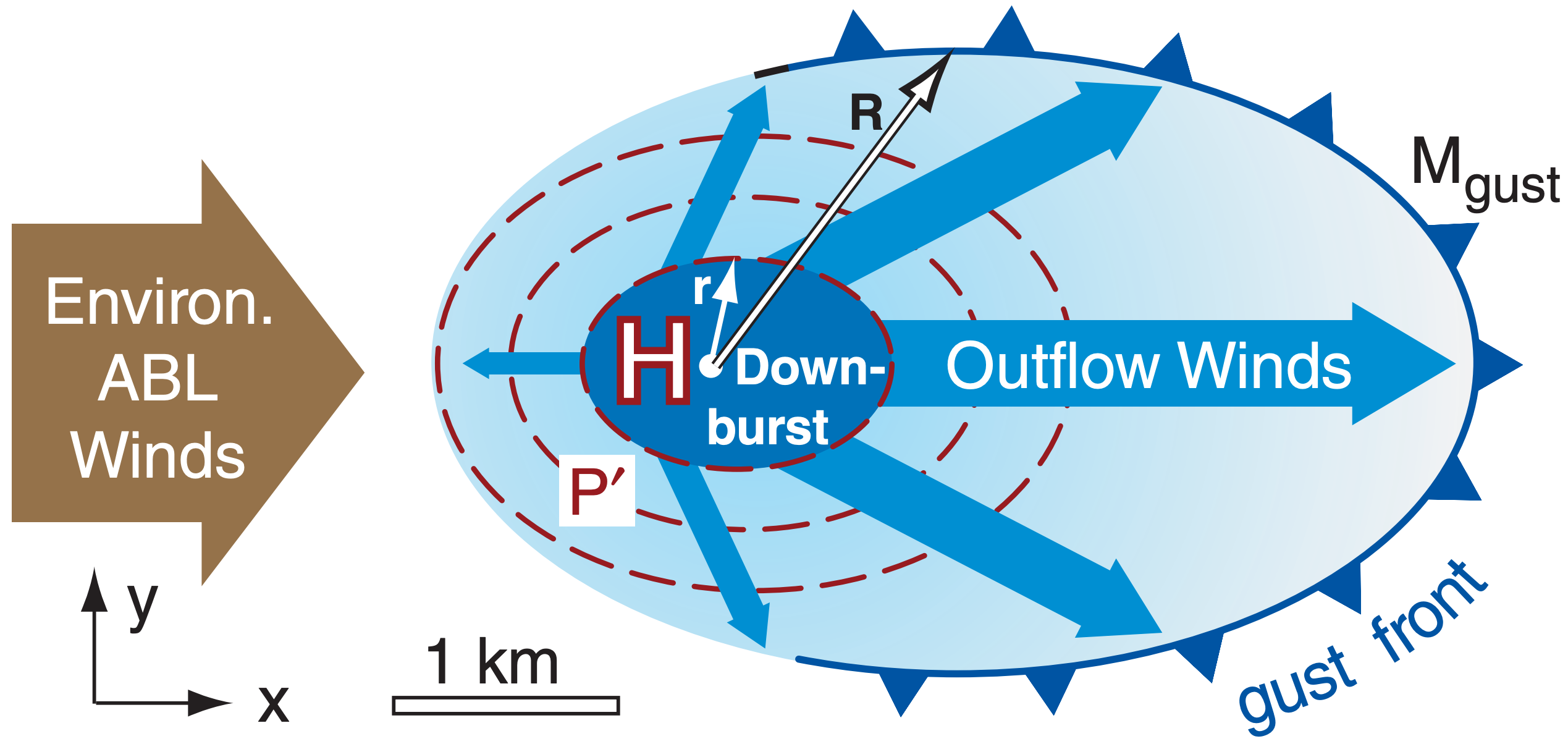
The outflow winds are accelerated by the perturbation-pressure gradient associated with the downburst mesohigh. Considering only the horizontal pressure-gradient force in Newton’s 2^nd Law (see the Forces & Winds Chapter), you can estimate the acceleration from

\(\ \begin{align} \frac{\Delta M}{\Delta t}=\frac{1}{\rho} \frac{P_{\max }^{\prime}}{r}\tag{15.13}\end{align}\)

where ∆M is change of outflow wind magnitude over time interval ∆t , ρ is air density, P’ _max is the pressure perturbation strength of the mesohigh, and r is the radius of the downburst (assuming it roughly equals the radius of the mesohigh).

Figure 15.18 Radar reflectivity from the San Angelo (SJT), Texas, USA, weather radar. White circle shows radar location. Thunderstorm cells with heavy rain (red & yellow) are over and northeast of the radar. Arrows show ends of gust front. Scale at right is radar reflectivity in dBZ. Radar elevation angle is 0.5°. Both figs. courtesy of the National Center for Atmospheric Research, based on National Weather Service radar data, NOAA.

Figure 15.19 Same as 15.18, but for Doppler velocity. Red, orange, and yellow colors are winds away from the radar (white circle), and light blue and turquoise are winds towards. Scale at right is speed in knots.

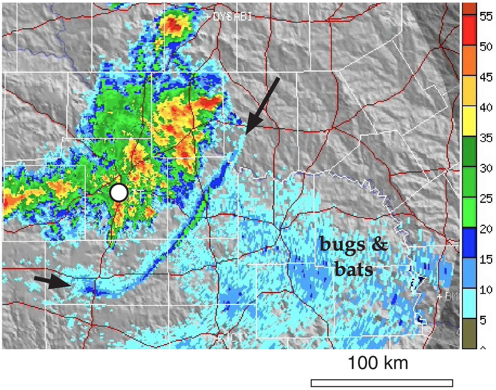
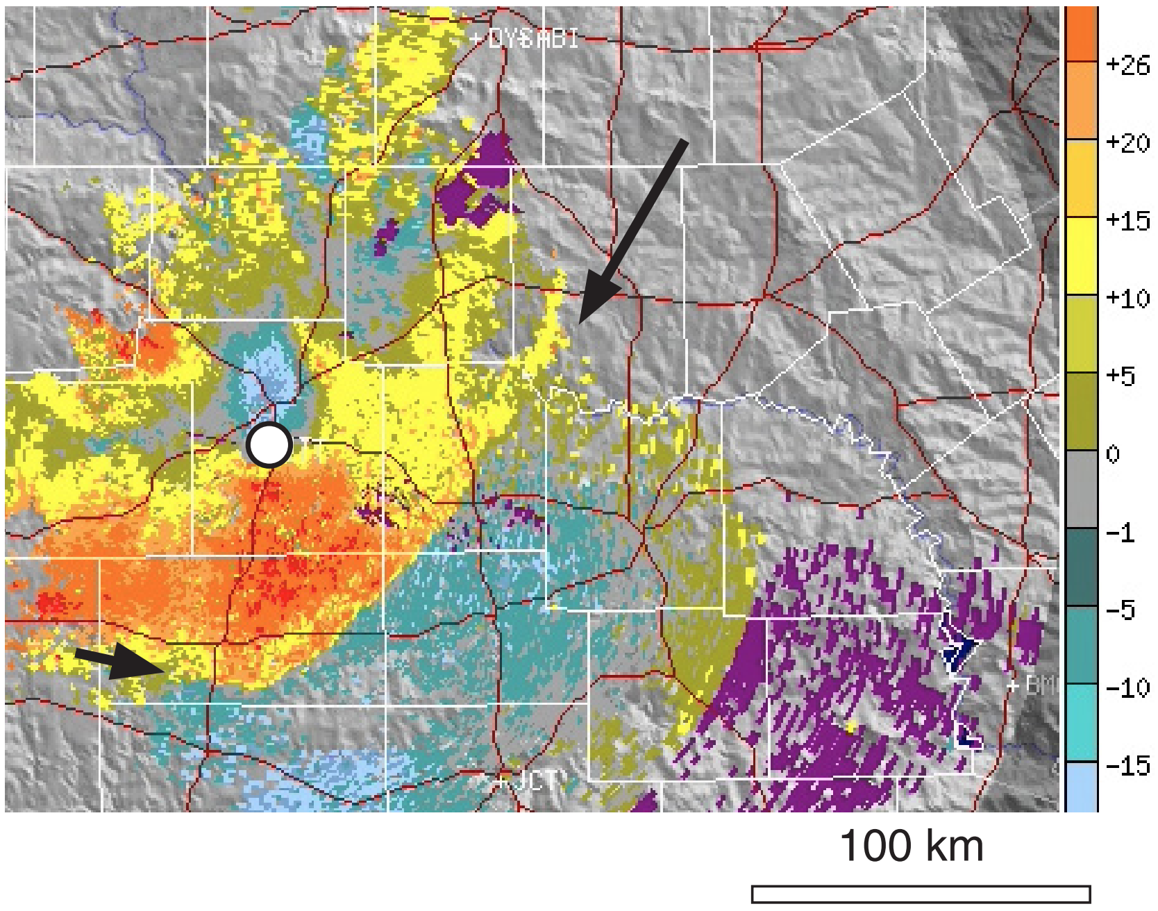
The horizontal divergence signature of air from a downburst can be detected by Doppler weather radar by the couplet of “toward” and “away” winds, as was shown in the Satellites & Radar chapter. Figs. 15.18 and 15.19 show a downburst divergence signature and gust front.

Downburst intensity (Table 15-2) can be estimated from the maximum radial wind speed M_max observed by Doppler radar in the divergence couplet, and from the max change of wind speed ∆M_max along a radial line extending out from the radar at any height below 1 km above mean sea level (MSL).

Gust front is the name given to the leading edge of the cold outflow air (Figs. 15.11 & 15.17). These fronts act like shallow (100 to 1000 m thick) cold fronts, but with lifetimes of only several minutes to a few hours. Gust fronts can advance at speeds ranging from 5 to 15 m s^–1, and their length can be 5 to 100 km. The longer-lasting gust fronts are often associated with squall lines or supercells, where downbursts of cool air from a sequence of individual cells can continually reinforce the gust front.

Temperature drops of 1 to 3 °C have been recorded as a gust front passes a weather station. As this cold, dense air plows under warmer, less-dense humid air in the pre-storm environmental atmospheric boundary layer (ABL), the ABL air can be pushed up out of the way. If pushed above its LCL, clouds can form in this ABL air, perhaps even triggering new thunderstorms (a process called propagation). The new storms can develop their own gust fronts that can trigger additional thunderstorms, resulting in a storm sequence that can span large distances.

Greater gust front speeds are expected if faster downbursts pump colder air toward the ground. The continuity equation tells us that the vertical inflow rate of cold air flowing down toward the ground in the downburst must balance the horizontal outflow rate behind the gust front. If we also approximate the outflow thickness, then we can estimate the speed M_gust of advance of the gust front relative to the ambient environmental air as

\(\ \begin{align} M_{g u s t}=\left[\frac{0.2 \cdot r^{2} \cdot\left|w_{d} \cdot g \cdot \Delta T_{v}\right|}{R \cdot T_{v e}}\right]^{1 / 3}\tag{15.14}\end{align}\)

where r is average downburst radius, R is average distance of the gust front from the downburst center, w_d is downburst speed, ∆T_v is virtual temperature difference between the cold-outflow and environmental air, and T_ve (K) is the environmental virtual temperature.

Sample Application

For a mesohigh of max pressure 0.5 kPa and radius 5 km, how fast will the outflow winds become during 1 minute of acceleration?

Find the Answer

Given: P’ _max = 0.5 kPa, r = 5 km, ∆t = 60 s

Find: ∆M = ? m s^–1

Solve eq. (15.13) for M. Assume ρ = 1.225 kg m^–3.

\(\Delta M=\frac{(60 \mathrm{s})}{\left(1.225 \mathrm{kg} / \mathrm{m}^{3}\right)} \cdot \frac{(0.5 \mathrm{kPa})}{(5 \mathrm{km})}=\underline{\mathbf{4 . 9} \mathrm{m} \mathrm{s}^{-1}}\)

Check: Physics OK. Units OK. Magnitude OK.

Exposition: In real downbursts, the pressure gradient varies rapidly with time and space. So this answer should be treated as only an order-of-magnitude estimate.

Table 15-2. Doppler-radar estimates of thunderstorm-cell downburst intensity based on either the maximum outflow wind speed or the maximum wind difference along a radar radial.
Intensity	Max radial-wind speed (m s^–1)	Max wind difference along a radial (m s^–1)
Moderate	18	25
Severe	25	40

In the expression above, the following approximation was used for gust-front thickness h_gust:

\(\ \begin{align} h_{g u s t} \approx 0.85 \cdot\left[\frac{T_{v e}}{\left|g \cdot \Delta T_{v}\right|}\left(\frac{w_{d} \cdot r^{2}}{R}\right)^{2}\right]^{1 / 3}\tag{15.15}\end{align}\)

As the gust front spreads further from the downburst, it moves more slowly and becomes shallower. Also, colder outflow air moves faster in a shallower outflow than does less-cold outflow air.

In dry environments, the fast winds behind the gust front can lift soil particles from the ground (a process called saltation). While the heavier sand particles fall quickly back to the ground, the finer dust particles can become suspended within the air. The resulting dust-filled outflow air is called a haboob (Fig. 15.20), sand storm or dust storm. The airborne dust is an excellent tracer to make the gust front visible, which appears as a turbulent advancing wall of brown or ocher color.

In moister environments over vegetated or rainwetted surfaces, instead of a haboob you might see arc cloud (arcus) or shelf cloud over (not within) an advancing gust front. The arc cloud forms when the warm humid environmental ABL air is pushed upward by the undercutting cold outflow air. Sometimes the top and back of the arc cloud are connected or almost connected to the thunderstorm, in which case the cloud looks like a shelf attached to the thunderstorm, and is called a shelf cloud.

When the arc cloud moves overhead, you will notice sudden changes. Initially, you might observe the warm, humid, fragrant boundary-layer air that was blowing toward the storm. After gust-front passage, you might notice colder, gusty, sharp-smelling (from ozone produced by lightning discharges) downburst air.

Figure 15.20 Sketches of (a) a haboob (dust storm) kicked up within the outflow winds, and (b) an arc cloud in the boundary-layer air pushed above the leading edge of the outflow winds (i.e., above the gust front). Haboobs occur in drier locations. Arc clouds occur in humid locations.

Sample Application

A thunderstorm creates a downburst of speed of 4 m s^–1 within an area of average radius 0.6 km. The gust front is 3°C colder than the environment air of 300 K, and is an average of 2 km away from the center of the downburst. Find the gust-front advancement speed and depth.

Find the Answer

Given: ∆T_v = –3 K, T_ve = 300 K, w_d = –4 m s^–1, r = 0.6 km, R = 2 km,

Find: M_gust = ? m s^–1, h_gust = ? m

Employ eq. (15.14): \(M_{g u s t}=
\left[\frac{0.2 \cdot(600 \mathrm{m})^{2} \cdot(-4 \mathrm{m} / \mathrm{s}) \cdot\left(-9.8 \mathrm{m} \cdot \mathrm{s}^{-2}\right) \cdot(-3 \mathrm{K})}{(2000 \mathrm{m}) \cdot(300 \mathrm{K})}\right]^{1/3}
=\underline{\mathbf{2.42 \mathrm{m} \mathrm{s}^{-1}}}
\)
Employ eq. (15.15):

\( h_{g u s t}=

0.85\left[\left(\frac{(-4 \mathrm{m} / \mathrm{s}) \cdot(600 \mathrm{m})^{2}}{(2000 \mathrm{m})}\right)^{2} \frac{(300 \mathrm{K})}{\left(-9.8 \mathrm{m} \cdot \mathrm{s}^{-2}\right) \cdot(-3 \mathrm{K})}\right]^{1 / 3} =\underline{\mathbf{174m}}\)

Check: Units OK. Physics OK.

Exposition: Real gust fronts are more complicated than described by these simple equations, because the outflow air can turbulently mix with the environmental ABL air. The resulting mixture is usually warmer, thus slowing the speed of advance of the gust front.