14.2: Thunderstorm Formation

14.2.1. Favorable Conditions

Four environmental (pre-storm) conditions are needed to form the strong moist convection that is a severe thunderstorm:

1. high humidity in the boundary layer,
2. nonlocal conditional instability
3. strong wind shear,
4. a trigger mechanism to cause lifting of atmospheric boundary-layer air.

Figure 14.22 Atmospheric conditions favorable for formation of strong thunderstorms.

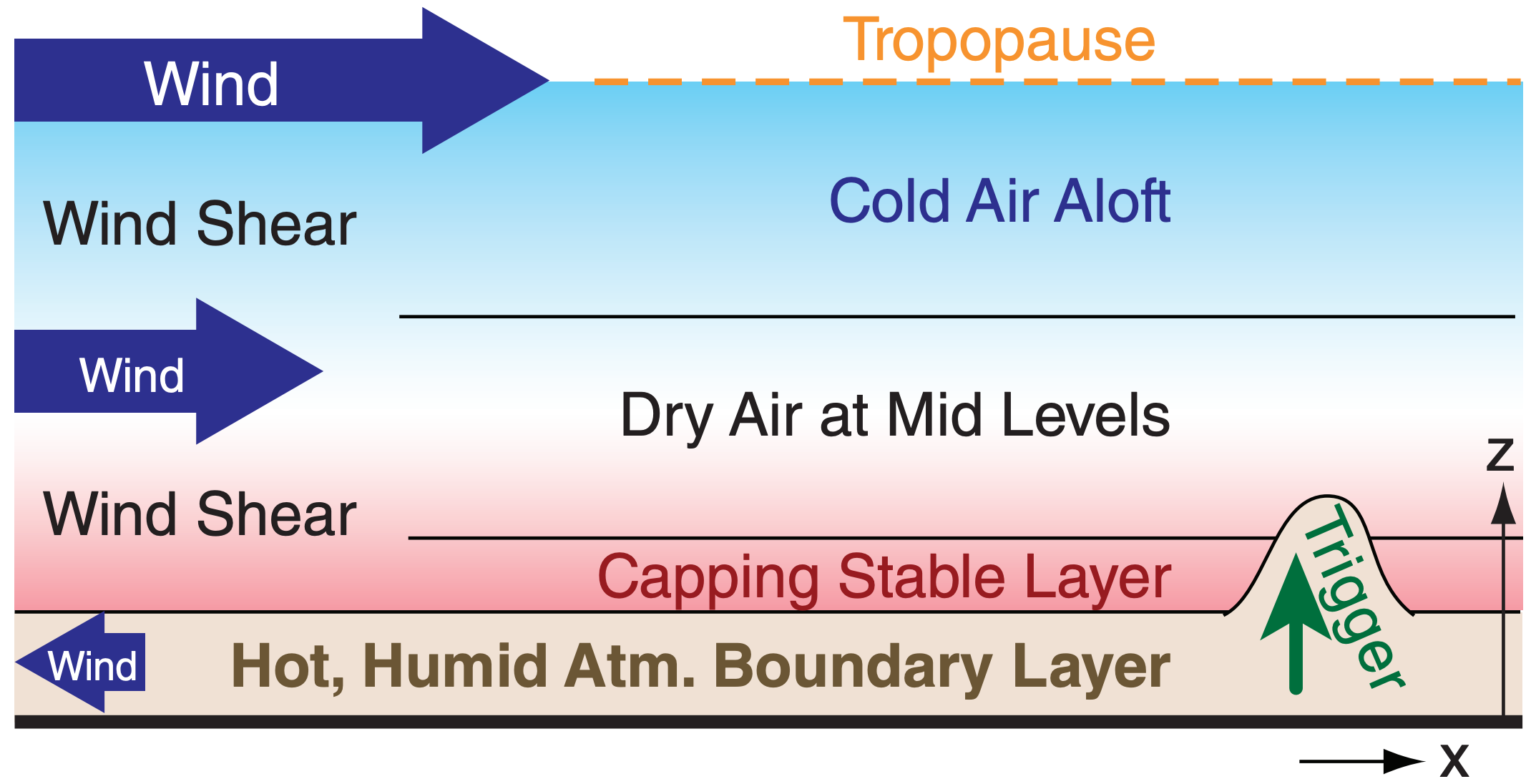
Fig. 14.22 illustrates these conditions. Meteorologists look for these conditions in the pre-storm environment to help forecast thunderstorms. We will examine each of these conditions in separate sections. But first, we define key convective altitudes that we will use in the subsequent sections to better understand thunderstorm behavior.

14.2.2. Key Altitudes

The existence and strength of thunderstorms depends partially on layering and stability in the prestorm environment. Thus, you must first obtain an atmospheric sounding from a rawinsonde balloon launch, numerical-model forecast, aircraft, dropsonde, satellite, or other source. Morning or early afternoon are good sounding times, well before the thunderstorm forms (i.e., pre-storm). The environmental sounding data usually includes temperature (T), dew-point temperature (T_d), and wind speed (M) and direction (α) at various heights (z) or pressures (P).

Figure 14.23 (a) Thermo diagram, with approximate height contours (z) added as nearly horizontal thin dashed lines (labeled at right). Sounding data plotted on this diagram will enable you to anticipate storm formation and strength. (b) Same as (a), but lighter colors to make it easier to write on.

Figure 14.24 Environmental sounding of temperature (T) and dew-point temperature (T_d) plotted on a thermo diagram. The mixed layer (ML), capping inversion (Cap), tropopause, troposphere, and stratosphere are identified. This example shows an early-afternoon pre-storm environment.

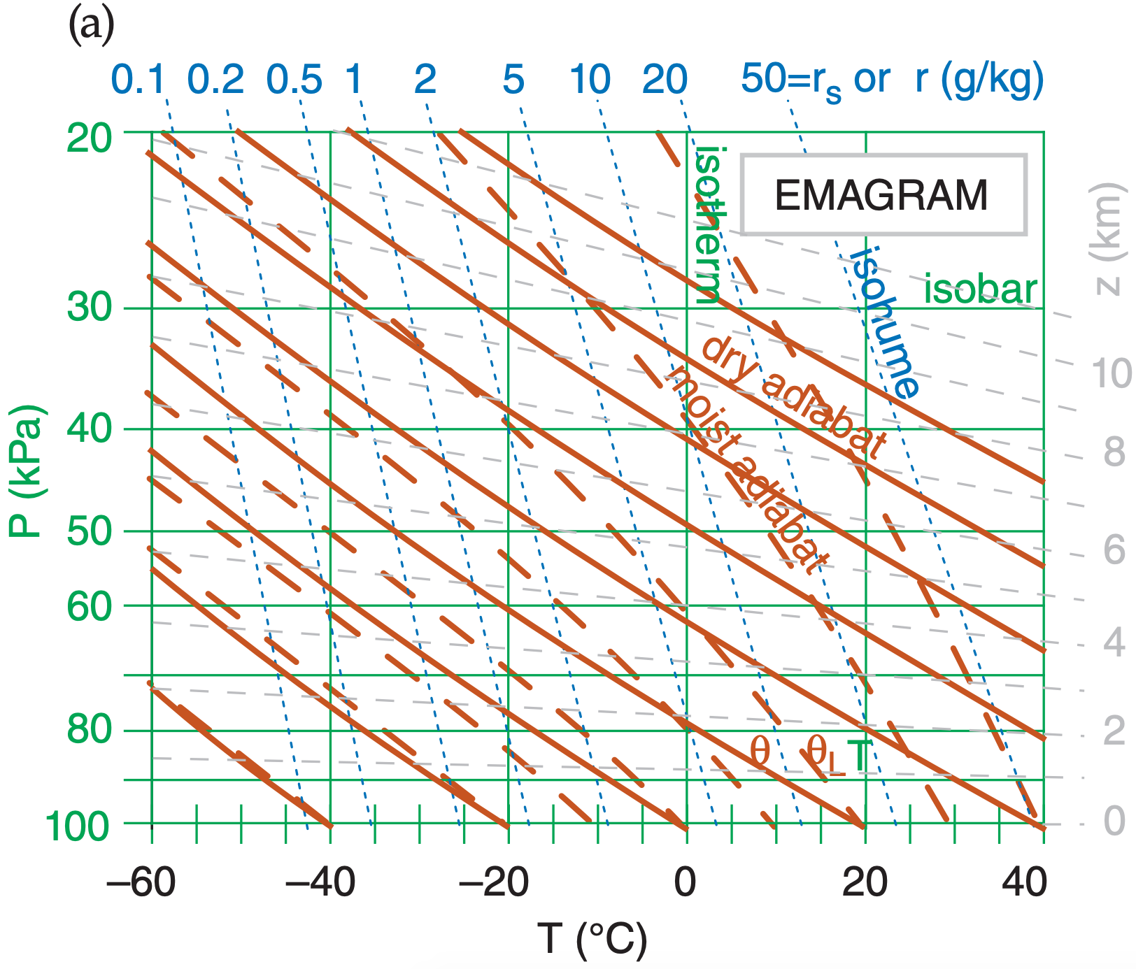
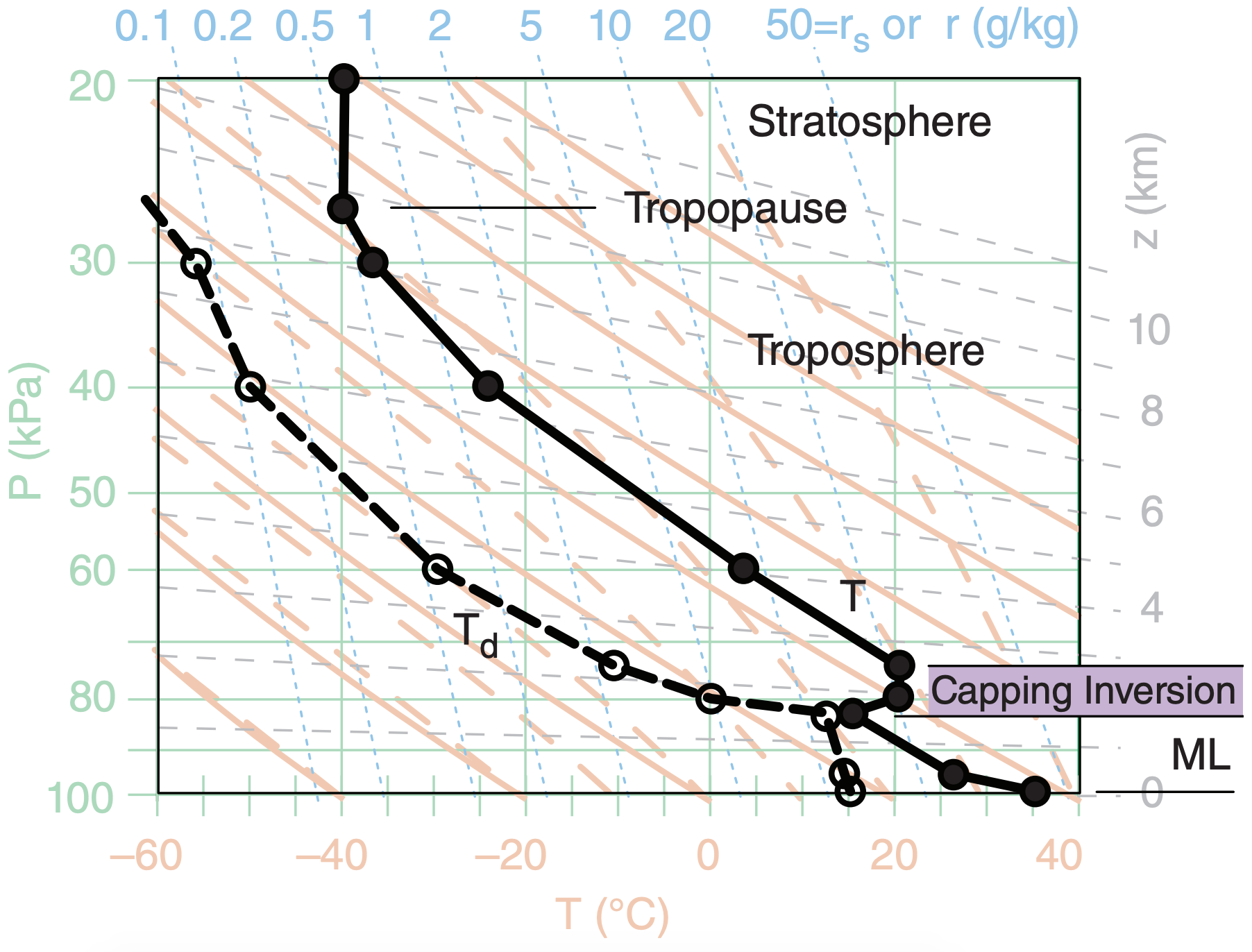
Plot the environmental sounding on a thermo diagram such as the Emagram of Fig. 14.23, being sure to connect the data points with straight lines. Fig. 14.24 shows a typical pre-storm (early afternoon) sounding, where T is plotted as black-filled circles connected with a thick black solid line, and T_d is plotted as white-filled circles connected with a thick black dashed line. The mixed layer (ML; i.e., the daytime turbulently well-mixed boundary layer), capping inversion, and tropopause are identified in Fig. 14.24 using the methods in the Atmospheric Stability chapter.

Daytime solar heating warms the Earth’s surface. The hot ground heats the air and evaporates soil moisture into the air. The warm humid air parcels rise as thermals in an unstable atmospheric boundary layer. If we assume each rising air parcel does not mix with the environment, then its temperature decreases dry adiabatically with height initially, and its mixing ratio is constant.

Figure 14.25 Afternoon pre-storm environmental air from near the surface (indicated with the circles), is hypothetically lifted as an air parcel to the top of the thermo diagram. Identified are the average mixed-layer height (z_i ), the lifting condensation level (LCL), the level of free convection (LFC), and the equilibrium level (EL).

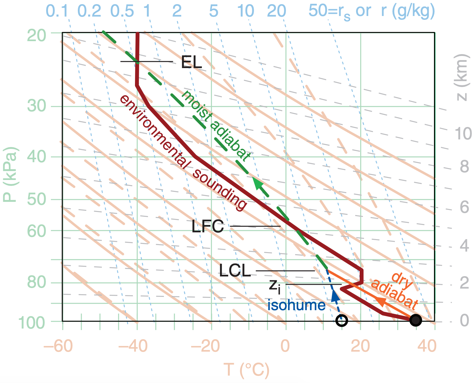
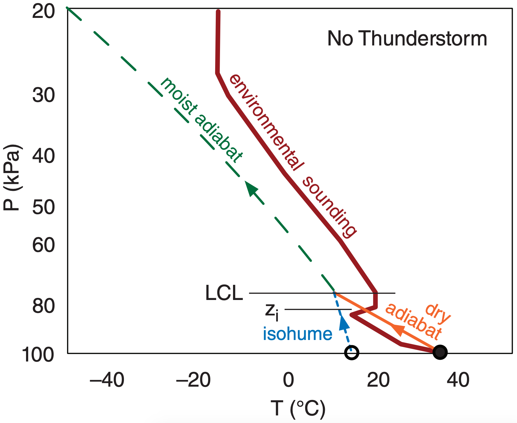
Fig. 14.25 shows how this process looks on a thermo diagram. The parcel temperature starts near the ground from the solid black circle and initially follows a dry adiabat (thin black solid line with arrow). The dew point starts near the ground from the open circle and follows the isohume (thin black dotted line with arrow).

Typically, the rising parcel hits the statically stable layer at the top of the mixed layer, and stops rising without making a thunderstorm. This capping temperature-inversion height z_i represents the average mixed-layer (ML) top, and is found on a thermo diagram where the dry adiabat of the rising parcel first crosses the environmental sounding (Fig. 14.25). In pressure coordinates, use symbol Pi to represent the ML top.

If the air parcel were to rise a short distance above z_i , it would find itself cooler than the surrounding environment, and its negative buoyancy would cause it sink back down into the mixed layer. On many such days, no thunderstorms ever form, because of this strong lid on top of the mixed layer.

But suppose an external process (called a trigger) pushes the boundary-layer air up through the capping inversion (i.e., above z_i ) in spite of the negative buoyancy. The rising air parcel continues cooling until it becomes saturated. On a thermo diagram, this saturation point is the lifting condensation level (LCL), where the dry adiabat first crosses the isohume for the rising parcel.

As the trigger mechanism continues to push the reluctant air parcel up past its LCL, water vapor in the parcel condenses as clouds, converting latent heat into sensible heat. The rising cloudy air parcel thus doesn’t cool as fast with height, and follows a moist adiabat on a thermo diagram (Fig. 14.25).

INFO • Cap vs. Capping Inversion

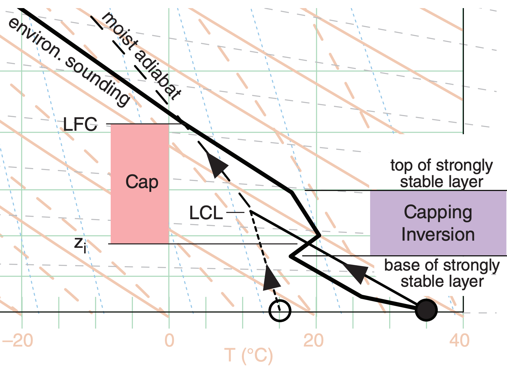
The strongly stable layer at the top of the daytime boundary layer (i.e., at the top of the mixed layer) is called the “capping inversion,” as sketched in the figure below (a modification of Fig. 14.25).

The region near the top of the mixed layer where the rising air parcel is colder than the environment is called the “cap.” It is this region between zi and the LFC that opposes or inhibits the rise of the air parcel, and which must be overcome by the external forcing mechanism. See the section later in this chapter on “Triggering vs. Convective Inhibition” for more details.

Figure 14.b Idealized pre-storm environmental sounding (thick solid line), plotted on the bottom right portion of an Emagram. Circles and lines with arrows show the rise of an air parcel from near the surface.

Even so, this cloudy parcel is still colder than the ambient environment at its own height, and still resists rising due to its negative buoyancy.

For an atmospheric environment that favors thunderstorm formation (Fig. 14.25), the cloudy air parcel can become warmer than the surrounding environment if pushed high enough by the trigger process. The name of this height is the level of free convection (LFC). On a thermo diagram, this height is where the moist adiabat of the rising air parcel crosses back to the warm side of the environmental sounding.

Above the LFC, the air parcel is positively buoyant, causing it to rise and accelerate. The positive buoyancy gives the thunderstorm its energy, and if large enough can cause violent updrafts.

Because the cloudy air parcel rises following a moist adiabat (Fig. 14.25), it eventually reaches an altitude where it is colder than the surrounding air. This altitude where upward buoyancy force becomes zero is called the equilibrium level (EL) or the limit of convection (LOC). The EL is frequently near (or just above) the tropopause (Fig. 14.24), because the strong static stability of the stratosphere impedes further air-parcel rise.

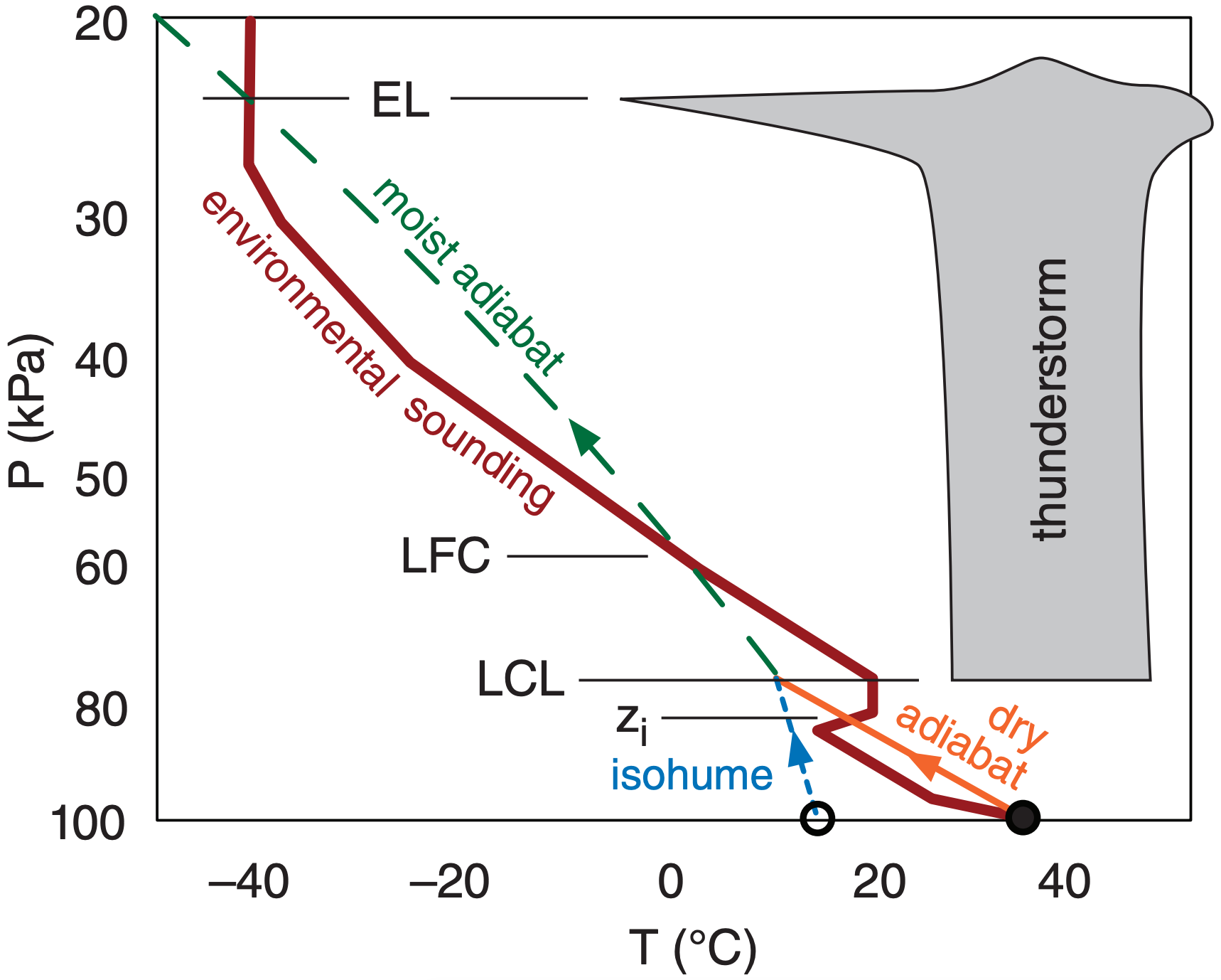
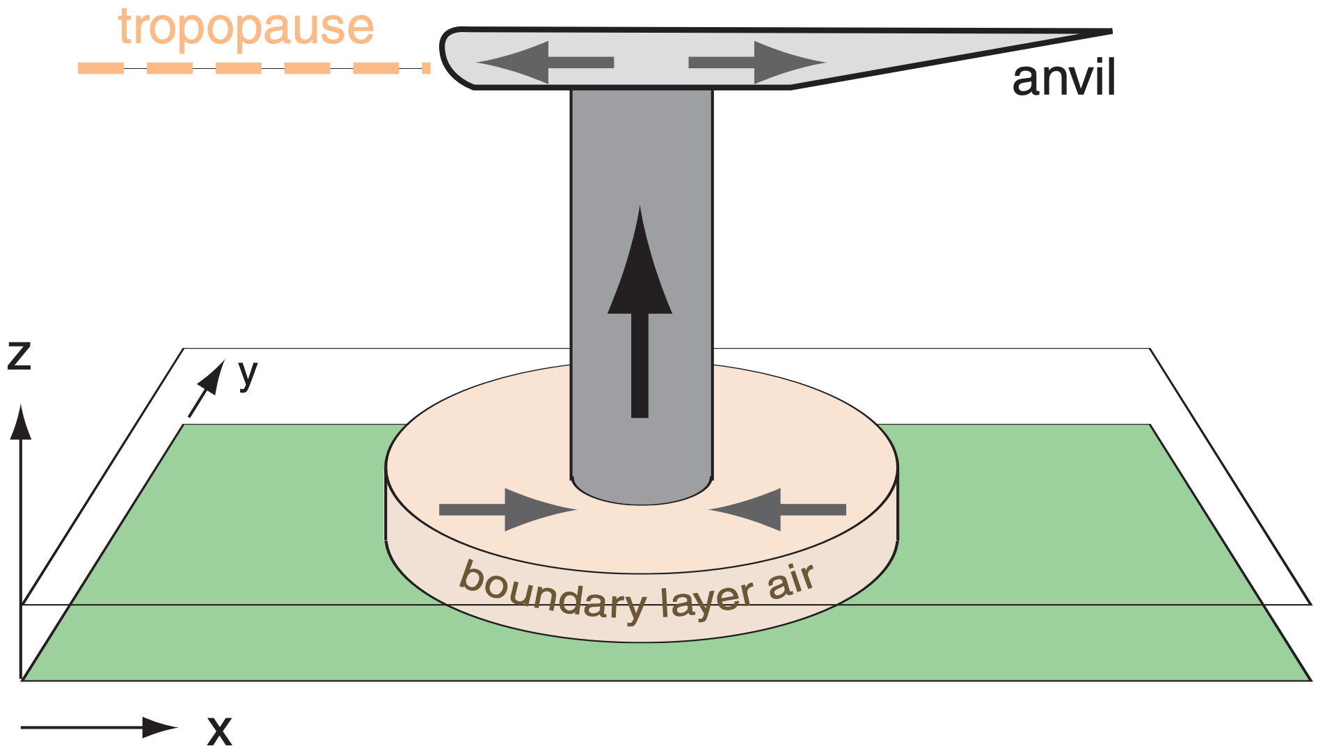
Thus, thunderstorm cloud-base is at the LCL, and thunderstorm anvil top is at the EL (Fig. 14.26). In very strong thunderstorms, the rising air parcels are so fast that the inertia of the air in this updraft causes an overshooting dome above the EL before sinking back to the EL. The most severe thunderstorms have tops that can penetrate up to 5 km above the tropopause, due to a combination of the EL being above the tropopause (as in Fig. 14.26) and inertial overshoot above the EL.

Figure 14.26 From Fig. 14.25, we infer that a thunderstorm could form with cloud top and base as sketched, if successfully triggered. Thunderstorm air parcels follow the thin diagonal solid and dashed lines, while the surrounding air is shown with the thick line.

For many thunderstorms, the environmental air between the EL and the LFC is conditionally unstable. Namely, the environmental air is unstable if it is cloudy, but stable if not (see the Atmospheric Stability chapter). On a thermo diagram, this is revealed by an environmental lapse rate between the dry- and moist-adiabatic lapse rates.

However, it is not the environmental air between the LFC and EL that becomes saturated and forms the thunderstorm. Instead, it is air rising above the LFC from lower altitudes (from the atmospheric boundary layer) that forms the thunderstorm. Hence, this process is a nonlocal conditional instability (NCI).

Frequently the LCL is below z_i . This allows fair-weather cumulus clouds (cumulus humilis) to form in the top of the atmospheric boundary layer (see the Sample Application at left). But a trigger mechanism is still needed to force this cloud-topped mixed-layer air up to the LFC to initiate a thunderstorm.

Sample Application

Plot this sounding on a full-size skew-T diagram (Atm. Stab. chapter), and estimate the pressure altitudes of the ML top , LCL, LFC, and EL for an air parcel rising from near the surface.

P (kPa)	T (°C)	Td (°C)
100	30	20.
96	25	.
80	10	.
70	15	.
50	–10	.
30	–35	.
20	–35	.

Find the Answer

Given: Data in the table above.

Find: P_i = ? kPa (= ML top), P_LCL = ? kPa, P_LFC = ? kPa, P_EL = ? kPa.

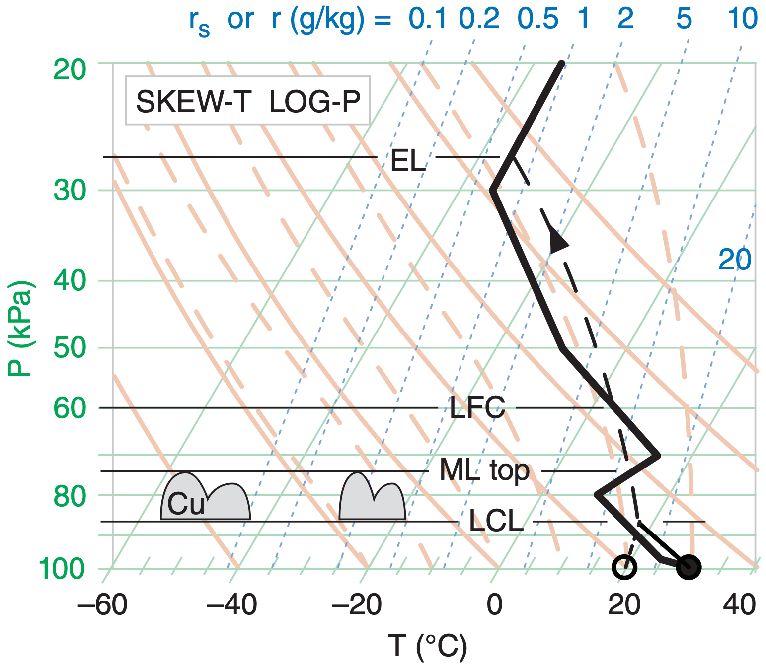
After plotting the air-parcel rise, we find:

P_i = 74 kPa, P_LCL = 87 kPa, P_LFC = 60 kPa, P_EL = 24 kPa.

Exposition: The LCL for this case is below the ML top. Thus, the ML contains scattered fair-weather cumulus clouds (cumulus humilis, Cu). If there is no external trigger, the capping inversion prevents these clouds from growing into thunderstorms.

Figure 14.27 An environmental sounding that does not favor thunderstorms, because the environmental air aloft is too warm. Emagram.

In many situations, no LFC (and also no EL) exists for an air parcel that is made to rise from the surface. Namely, the saturated air parcel never becomes warmer than the environmental sounding (such as Fig. 14.27). Such soundings are NOT conducive to thunderstorms.

Sample Application

How much energy does an air-mass thunderstorm release? Assume it draws in atmospheric boundary layer (ABL, or BL) air of T_d = 21°C & depth ∆z_BL = 1 km (corresponding roughly to ∆P_BL = 10 kPa), and that all water vapor condenses. Approximate the cloud by a cylinder of radius R = 5 km and depth ∆z = 10 km with base at P = 90 kPa & top at P = 20 kPa.

Find the Answer

Given: R = 5 km, ∆z = 10 km, T_d = 21°C, ∆z_BL = 1 km, ∆P_BL = 10 kPa, ∆P_storm = 90 – 20 = 70 kPa

Find: ∆Q_E = ? (J)

Use eq. (3.3) with L_v = 2.5x10⁶ J·kg^–1, and eq. (4.3)

\(\ \begin{align} \Delta Q_{E}=L_{v} \cdot \Delta m_{w a t e r}=L_{v} \cdot r \cdot \Delta m_{a i r}\tag{a}\end{align}\)

where r ≈ 0.016 kg_water·kg_air^–1 from thermo diagram.

But eq. (1.8) ∆P = ∆F/A and eq. (1.24) ∆F = ∆m·g give:

\(\ \begin{align} \Delta m_{a i r}=\Delta P \cdot A / g\tag{b}\end{align}\)

where A = surface area = πR².

For a cylinder of air within the ABL, but of the same radius as the thunderstorm, use eq. (b), then (a):

∆m_air = (10 kPa)·π·(5000m)²/(9.8 m s^–2)= 8x10⁸ kg_air

∆Q_E=(2.5x10⁶ J·kg^–1)(0.016 kg_water·kg_air^–1)·(8x10⁸ kg_air) = 3.2x10¹⁵ J

Given the depth of the thunderstorm (filled with air from the ABL) compared to the depth of the ABL, we find that ∆P_storm = 7·∆P_BL (see Figure).

Thus, ∆Q_{E storm} = 7 ∆Q_{E BL}

∆Q_{E storm} = 2.24x10¹⁶ J

Check: Physics OK. Units OK. Values approximate.

Exposition: A one-megaton nuclear bomb releases about 4x10¹⁵ J of heat. This hypothetical thunderstorm has the power of 5.6 one-megaton bombs.

Actual heat released in a small thunderstorm is about 1% of the answer calculated above. Reasons include: T_d < 21°C; storm entrains non-ABL air; and not all of the available water vapor condenses. However, supercells continually draw in fresh ABL air, and can release more heat than the answer above. Energy released differs from energy available (CAPE). For another energy estimate, see the “Heavy Rain” section of the next chapter.